The Density Cluster Tree: A Guest Post

Today, we have a guest post by Sivaraman Balakrishnan. Siva is a graduate student in the School of Computer Science. The topic of his post is an algorithm for clustering. The algorithm finds the connected components of the level sets of an estimate of the density. The algorithm — due to Kamalika Chaudhuri and Sanjoy DasGupta— is very simple and comes armed with strong theoretical guarantees.

Aside: Siva’s post mentions John Hartigan. John is a living legend in the field of statistics. He’s done fundamental work on clustering, Bayesian inference, large sample theory, subsampling and many other topics. It’s well worth doing a Google search and reading some of his papers.

Before getting to Siva’s post, here is a picture of a density and some of its level set clusters. The algorithm Siva will describe finds the clusters at all levels (which then form a tree).

THE DENSITY CLUSTER TREE
by
SIVARAMAN BALAKRISHNAN

1. Introduction

Clustering is widely considered challenging both practically and theoretically. One of the main reasons for this is that often the true goals of clustering are not clear and this makes clustering seem poorly defined.

One of the most concrete and intuitive ways to define clusters when data are drawn from a density ${f}$ is on the basis of level sets of ${f}$ , i.e. for any ${\lambda}$ the connected components of

$\displaystyle \{x: f(x) \geq \lambda\}$

form the clusters at level ${\lambda}$ . This leaves the question of how to select the “correct” ${\lambda}$ , and typically we simply sweep over ${\lambda}$ and present what is called the density cluster tree.

However, we usually do not have access to ${f}$ and would like to estimate the cluster tree of ${f}$ given samples drawn from ${f}$ . Recently, Kamalika Chaudhuri and Sanjoy Dasgupta (henceforth CD) presented a simple estimator for the cluster tree in a really nice paper: Rates of convergence for the cluster tree (NIPS, 2010) and showed it was consistent in a certain sense.

This post is about the notion of consistency, the CD estimator, and its analysis.

2. Evaluating an estimator: Hartigan’s consistency

The first notion of consistency for an estimated cluster tree was introduced by J.A. Hartigan in his paper: Consistency of single linkage for high-density clusters (JASA, 1981).

Given some estimator ${\Theta_n}$ of the cluster tree of ${f}$ (i.e. a collection of hierarchically nested sets), we say it is consistent if:

For any sets ${A,A^\prime \subset \mathbb{R}^d}$ , let ${A_n}$ (respectively ${A^\prime_n}$ ) denote the smallest cluster of ${\Theta_n}$ containing the samples in ${A}$ (respectively ${A}$ ). ${\Theta_n}$ is consistent if, whenever ${A}$ and ${A^\prime}$ are different connected components of ${\{x : f(x) \geq \lambda \}}$ (for some ${\lambda > 0}$ ), ${P(A_n}$ is disjoint from ${A^\prime_n) \rightarrow 1}$ as ${n \rightarrow \infty}$ .

Essentially, we want that if we have two separated clusters at some level ${\lambda}$ then the cluster tree must reflect this, i.e. the smallest clusters containing the samples from each of these clusters must be disconnected from each other.

To give finite sample bounds, CD introduced a notion of saliently separated clusters and showed that these clusters can be identified using a small number of samples (as a by-product their results also imply Hartigan consistency for their estimators). Informally, clusters are saliently separated if they satisfy two conditions.

Separation in ${\mathbb{R}^d}$ : We would expect that clusters that are two close cannot be identified in a finite sample.
Separation in the density ${f}$ : There should a sufficiently big region of low density separating the clusters. Again, we would expect that if the “bridge” between the clusters doesn’t dip enough then we might (incorrectly) conclude they are the same cluster from a finite sample.

3. An algorithm

The CD estimator is based on the following algorithm:

INPUT: ${k}$
For ${r = [0,\infty)}$ , discard all points with ${r_k(x) > r}$ where ${r_k(x)}$ is the distance to the ${k^{\rm th}}$ nearest neighbor of ${x}$ . Connect ${x,y}$ if ${||x-y|| \leq \alpha r}$ , to form ${G(r)}$ .
OUTPUT: Return connected components of ${G(r)}$ .

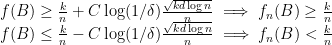
CD show that their estimator is consistent (and give finite sample rates for saliently separated clusters) if we select ${k \sim d \log n}$ and ${\alpha \geq \sqrt{2}}$ .

It is actually true that any density estimate that is uniformly close to the true density can be used to construct a Hartigan consistent estimator. However, this involves finding the connected components of the level sets of the estimator, which can be hard. The nice thing about the CD estimator is that it is completely algorithmic.

3.1. Detour 1: Single linkage

Single linkage is a popular linkage clustering algorithm, and essentially corresponds to the case of ${\alpha = 1, k = 2}$ . Given its popularity an important question to ask is whether the single linkage tree is Hartigan consistent. This was answered by Hartigan in his original paper, affirmatively for ${d=1}$ but negatively for ${d > 1}$ .

The main issue is an effect called “chaining” which causes single linkage to merge clusters before fully connecting up the clusters within themselves. The reason for this is that single-linkage is not sufficiently sensitive to the density separation, i.e. even if there is a region of low density between two clusters single linkage might form a “chain” across it because it is mostly oblivious to the density of the sample.

Returning to the CD estimator: one intuitive way to understand the estimator is to observe that for a fixed ${r}$ , the first step discards points on the basis of their distance to their ${k}$ -th NN. This is essentially cleaning the sample to remove points in regions of low-density (as measured by a ${k}$ -NN density estimate). This step makes the algorithm density sensitive and prevents chaining.

4. Analysis

So how does one analyze the CD estimator? We essentially need to show that for any two saliently separated clusters at a level ${\lambda}$ , there is some radius ${r}$ at which:

We do not clean out any points in the clusters.
The clusters are internally connected at the radius ${\alpha r}$ .
The clusters are mutually separated at this radius.

To establish each of these we will first need to understand how the ${k}$ -NN distance of the sample points behave given a finite sample.

4.1. Detour 2: Uniform large deviation inequalities

As before we are given ${n}$ random samples ${\{X_1, \ldots, X_n\}}$ from a density ${f}$ on ${\mathbb{R}^d}$ . Let’s say we are interested in a measurable subset ${A}$ of the space ${\mathbb{R}^d}$ . A fundamental question is: How close is the empirical mass of ${A}$ to the true mass of ${A}$ ? i.e. we would like to relate the quantities ${f_n(A) = n^{-1}\sum_{i=1}^n \mathbb{I} (X_i \in A)}$ and ${f(A)\equiv \int_A f(x)dx}$ . Notice that this is essentially the same as the question: if I toss a coin with bias ${f(A)}$ , ${m}$ times, on average how many heads will I see?

A standard way to answer these questions quantitatively is using a large deviation inequality like Hoeffding’s inequality. Often we have multiple sets ${\mathcal{A} = \{A_1, \ldots, A_N\}}$ and we’d like to relate ${f_n(A_i)}$ to ${f(A_i)}$ for each of these sets. One quantity we might be interested in is

$\displaystyle \Delta = \sup_i | f_n(A_i) - f(A_i)|$

and quantitative estimates of ${\Delta}$ are called uniform convergence results.

One surprising fact is that even for infinite collections of sets ${\mathcal{A}}$ we can sometimes still get good bounds on ${\Delta}$ if we can control the complexity of ${\mathcal{A}}$ . Typical ways to quantify this complexity are things like covering numbers, VC dimension etc.

To conclude this detour here is an example of this in action. Let ${\mathcal{A}}$ be the collection of all balls (with any center and radius) in ${\mathbb{R}^d}$ , if ${k \geq d \log n}$ then with probability ${1-\delta}$ , for any ${B \in \mathcal{A}}$

$\displaystyle \begin{array}{rcl} f(B) \geq \frac{k}{n} + C \log (1/\delta) \frac{\sqrt{kd \log n}}{n} \implies f_n(B) \geq \frac{k}{n} \\ f(B) \leq \frac{k}{n} - C \log (1/\delta) \frac{\sqrt{kd \log n}}{n} \implies f_n(B) < \frac{k}{n} \end{array}$

The inequalities above are uniform convergence inequalities over the sets of all balls in ${\mathbb{R}^d}$ . Although this is an infinite collection of sets it has a small VC dimension of ${d+1}$ , and this lets us uniformly relate the true and empirical mass of each of these sets.

In the context of the CD estimator what this detour assures us is that ${k}$ -NN distance of the every sample point is close to the “true” ${k}$ -NN distance. This lets us show that for an appropriate radius we will not remove any point from a high-density cluster (because it will have a small ${k}$ -NN distance) or that we will remove all points in the low-density region that separates salient clusters (because they will have large ${k}$ -NN distance). Results like this let us establish consistency of the CD estimator.

References.

Chaudhuri, K. and DasGupta, S. (2010). Rates of convergence for the cluster tree. Advances in Neural Information Processing Systems, 23, 343–351.

Hartigan, J. (1981). Consistency of single linkage for high-density clusters. Journal of the American Statistical Association, 76, 388-394.

4 Comments

Christian Hennig

Posted November 24, 2012 at 1:08 pm | Permalink

This is nice and well explained. A problem with this kind of consistency result, though, is that “k needs to increase as d log n” doesn’t tell us much about how to choose k in a real situation with n and d fixed. I suspect this choice may make quite some difference to the result. Are there recommendations (and a sound rationale for making them)?
- Sivaraman Balakrishnan
  
  Posted November 24, 2012 at 4:35 pm | Permalink
  
  I think that’s a very good question. I don’t think there is a conclusive answer yet but here are some half-baked ideas from Larry, Aarti (http://www.cs.cmu.edu/~aarti/), Alessandro (http://www.stat.cmu.edu/~arinaldo/) and others:
  
  1. Something like a Lepski-type method: Here is a paper by Singh, Scott, Nowak where they show minimizing a criterion with a BIC-like complexity penalty works (in theory) for bin width selection for histograms with Hausdorff loss. There is a similar criterion to minimize for k-NN estimators, for a fixed level set, which preserves the consistency results for that level set
  
  Click to access 0908.3593v1.pdf
  
  2. In practice one could try to bootstrap the sample and pick a value of k for which the clustering is stable across the various subsamples. I think you have to have a good way to compare trees across the subsamples. There are some heuristics including kernels on trees for that.
  
  3. Just like drawing a tree gets around the problem of having to choose a level set, you can also get around having to pick k by varying it (from 0 to n). This is no longer a tree so visualizing it is challenging, but it might be possible to develop some notion of persistent (across various values of k) clusters and just try to visualize those.
Matías

Posted November 29, 2012 at 10:20 pm | Permalink

Nice in it’s simplicity. It seems to be connected with the manifold learning named previously in this blog ¿isn’t it? (drawing balls over each remaining data point), and just these days I think I’m beginning to understand some of the usefulness of (in some cases) infering manifolds rather than response functions.
- Sivaraman Balakrishnan
  
  Posted December 1, 2012 at 11:37 am | Permalink
  
  Yes, I think you’re right and that is a good point. In some sense the (Haudorff/homology) manifold estimation problem is like estimating the support of the density (when there is no noise) and here you’re trying to estimate all level sets but with a different loss function.

One Trackback

By Implementing the Chaudhuri-Dasgupta density cluster tree | Statistics a.e. on July 11, 2013 at 5:31 pm

[…] few months ago Siva Balakrishnan wrote a nice post on Larry Wasserman’s blog about the Chaudhuri-Dasgupta algorithm for estimating a density […]

Normal Deviate