Recently, there was a discussion on stack exchange about an example in my book. The example is a paradox about estimating normalizing constants. The analysis of the problem in my book is wrong; more precisely, the analysis is my book is meant to show that just blindly applying Bayes’ rule does not always yield a correct posterior distribution.
This point was correctly noted by a commenter at stack exchange who uses the name “Zen.” I don’t know who Zen is, but he or she correctly identified the problem with the analysis in my book.
However, it is still an open question how to do the analysis properly. Another commenter, David Rohde, identified the usual proposal which I’ll review below. But as I’ll explain, I don’t think the usual answer is satisfactory.
The purpose of this post is to explain the paradox and then I want to ask the question: does anyone know how to correctly solve the problem?
The example, by the way, is due to my friend Ed George.
1. Problem Description
The posterior for a parameter 

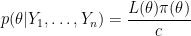
where 

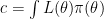

In complicated models, especially where 
In many cases we can use simulation methods (such as MCMC) to draw a sample 
More generally, suppose that

where 


2. Frequentist Estimator
We can use the sample to compute a density estimator 


where 
This is only one possible estimator. In fact, there is much research on the problem of finding good estimators of
As David Rohde notes on stack exchange, there is a certain irony to the fact the Bayesians use frequentist methods to estimate the normalizing constant of their posterior distributions.
3. A Bogus Bayesian Analysis
Let’s restate the problem. We have a sample 

In my book, I consider the following Bayesian analysis. The analysis is wrong, as I’ll explain in a minute.
We have an unknown quantity 

where we dropped the terms 
The “posterior” 
The point of the example was to point out that blindly applying Bayes rule is not always wise. As I mentioned earlier, Zen correctly notes that my application of Bayes rule is not valid. The reason is that, I acted as if we had a family of densities 


4. A Correct Bayesian Analysis?
The usual Bayesian approach that I have seen is to pretend that the function 
Christian Robert discussed the problem on his blog. If I understand what Christian has written, he claims that this cannot be considered a statistical problem and that we can’t even put a prior on
5. The Answer Is …
So what is a valid Bayes estimator of
I want to emphasize that this is not meant in any way as a critique of Bayes. I really think there should be a good Bayesian estimator here but I don’t know what it is.
Anyone have any good ideas?

58 Comments
I would recommend Kong, A., McCullagh, P. Meng, X.-L., Nicolae, D. and Tan, Z. (2003). A Theory of Statistical Models for Monte Carlo Integration (with Discussion). JRSS-B, 65, 585-618. Their trick is to place the uncertainty in the base measure for f, not the constant c. This appears to be a more fruitful approach.
Thanks. I meant to include that reference too.
But again, I don’t think it provides a real solution.
It seems very similar to the `forget you know g’ approach.
–LW
The problem here seems to be that knowledge of g(theta), in principle, fixes c. That is, there exists no valid prior distribution in which we know the function g() and know the constraint $c = \int f(\theta)d\theta$ but don’t know c. (A prior here is a distribution over at least g, c, and theta, and I am taking “knowing something” to mean that the something is true wp1 in our prior.) Without being able to select a prior which expresses the uncertainty we want to reason about, it seems difficult to set up a Bayesian inference problem.
This paradox seems like an instance of a larger (and really interesting) question: is it possible to use Bayesian inference to reason about the outcome of a known, deterministic computation from known inputs? To do so, it seems like we either have to change my definition above of “knowing something” (but I’m not sure what to replace it with) or change the rules of inference (which seems hard too).
Are inference (frequentist, Bayesian, Fiducial,…) tools appropriate to solve well defined equalities? I guess this is what Geoff meant by “reason about the outcome of a known, deterministic computation from known inputs”. I have in mind the estimation of multinomial probabilities; any acceptable estimation method will force the probabilities to sum to one.
I also wonder if independence of the data is a problem? Since c is fixed and well defined, why one expect for different samples to convey different information about it?
I guess Larry’s point is that if we can do Bayesian inference about, say, the speed of light (which has a fixed but unknown value), why can’t we do Bayesian inference about other fixed but unknown values, such as a partition function? The method that Larry described doesn’t work, but that doesn’t mean that there isn’t one that would.
Importance sampling can be used to estimate partition functions (the annealed versions work better, but let’s ignore that here). Suppose we have the results of several importance sampling runs using different reference distributions and different numbers of samples, and we want to combine them somehow. A Bayesian method would actually seem to be a sensible way of combining several such runs, because given a value c for the partition function, we can calculate the “likelihood” of each importance sampling run. All we need is a prior over c.
Hmm, calculating the “likelihood” of each importance sampling run is not as easy as I thought (that will teach me to post before checking!) but at least approximating this “likelihood” seems possible. For example, one could build a histogram from multiple runs with the same parameters. (I’m not claiming this is efficient; only that it is possible to come up with a “likelihood” that would let us do Bayesian inference for the partition function c).
This doesn’t work either. I’m stopping before I make more mistakes!
I would say there is a difference between knowing a variable in a representation, but not in another. For instance, you can define a number x* as argmax f(x) – we “know” what x* is, but we might not know it in another representation: its numerical value. Unsurprinsingly, there are Bayesian ways of solving optimization problems, solving differential equations, and etc. other numerical problems. Integration is just another numerical problem. And yes, I disagree with Christian. Isn’t knowing the average vote preference of every American just a matter of going to each of them and asking it? Yes, it is harder than getting a computer to evaluate a function at a particular position, but by the end of the day this is about providing estimates of quantities we could not measure due to lack of resources. I don’t see a clash between assuming one knows g(x) in its mathematical definition but not in its numerical form – just because we might immediately compute the numerical value of g(x) for any particular value of x, it is fair to say we do not know what the value of g(x) is for its infinitely many instances.
I think what this very interesting example points to is that there is a tension in the idea of Bayesian approximation.
If you condition on everything you know then there can be no approximation. If instead you explicitly condition on e.g. Monte Carlo samples or evaluations of the posterior at certain points then you need to average over things that you in principle “know” and if you define Bayesian statistics as condition on everything, then this is no longer Bayesian statistics.
If non-Bayesian methods seem to have fewer problems here, it comes from a comfort in throwing away information that you really know. This is both good and bad.
I think practical Bayesian statistics cannot be fully conditional.
Although I don’t claim to understand it I think Bayes linear statistics is an interesting development. Despite the name it is quite a radical idea….
http://books.google.com.au/books?hl=en&lr=&id=34Z46xxlIfsC&oi=fnd&pg=PR18&dq=bayes+linear+statistics&ots=R2pmdRUUNd&sig=Zw3FMpIWwRKXE22aSiC6ev8c_Co
Thanks for the comment.
I’m not sure why the density estimator approach
is throwing anything away
LW
(Thanks for mentioning my little comment on your blog, I was thrilled!)
The density estimator approach uses a Monte Carlo method which internally evaluates the likelihood at a finite number of points. Even though the likelihood/posterior is known everywhere the answer is just based upon a few points, so I think both are ignoring most of the posterior/likelihood and making smoothing assumptions.
In order to have a Bayesian method you will need to have a joint distribution over $c$ and something else that you will condition upon, perhaps a finite number of evaluations of $g()$. What it means to know or have a prior on $c$ or $g$ is of course challenging philosophically. I think it is reasonable to say if $c$ is unknown then so is $g()$…. but it is a challenging area… What is the prior on $g()$? Should it be related to $\pi()$? I think so …. but that may not lead to an easier computation….
Moving to a bigger picture, why use “Bayes Numerical Methods” at all?
I think conventional applied Bayesian statistics is normally considered to be an approximation to a fully conditional analysis.
Bayesian statistics computed using Bayes numerical methods on the other hand is not fully conditional, but it is also no longer approximate. i.e. rather than conditioning on the likelihood everywhere it is just conditioned on in a few places… If this could be showed to be generally possible, it might be useful…. This type of Bayesian statistics would need to borrow some ideas from non-Bayesian statistics and would inherit some of these weakness (but it would be computable).
Another way to look at it is that a traditional applied Bayesian analysis with MCMC has both frequentist Monte Carlo uncertainty and Bayesian statistical uncertainty. It would be nice to combine these sensibly, perhaps to motivate decision theoretic structure that included decisions to apply more computation or gather more data or present the result now.
Isn’t it well-known that use of e.g. Monte Carlo methods gives a approximate Bayesian inference, although the approximation is done in a non-Bayesian framework?
I find the example very unsatisfying. One might as well ask for a Bayesian estimator of the 10th decimal place of pi (or pi raised to some power based on the known data, if you prefer). There’s nothing statistical to do. An equivalent for the speed of light – Mark’s example – is to exactly specify all the parameters for a complete, deterministic model for the universe, and then to see what value of $c$ drops out of there. No statistics is involved, just lots of calculation.
Yes but we really need to know c and we have data.
What do we do?
If the samples are drawn from the prior then the monte carlo willl converge to the posterior. this is the markov chain monte carlo approach. the reason c is usually called a “normalizing” constant is because people don’t know how or are unwilling to try to specify it a priori. The crude approach is to make it a uniform distribution, then it looks like a normalizing constant. If your prior knowledge of the data is weak, it probably doesn’t matter; but it is illogical to assign priors in an ad hoc fashion.
No the sample is drawn from the posterior not the prior
(using MCMC). Yes we can use averaging (such as importance sampling etc)
but that misses the point. We want to write down a valid posterior for c.
What Klaus Mosegaard and Albert Tarantola (among others) discovered is that if you draw samples from the prior and then weight with the likelihood function then you never have to simulate for models with low a priori probability. Of coures, we had models with thousands of parameters and millions of data, so efficiency was crucial. If you sample directly from the posterior, most of these models will have low a priori probability. In principle you get the same result either way, but one is vastly more efficient.
the issue of c is completely different. if you have a prior on the model you must have a prior on the data. at least that’s how alll the bayesians I know interpret things. If you have an instrument that measures up to +/- 1 volt and you get 10 volts out, the datum has zero a priori probability.
I agree, the sense in which we know c is very unsatisfying. Intuitively, it makes a lot of sense to say that I know c in one representation but not another — but I don’t know how to make that statement in a formal Bayesian way. That is, I think Bayesian reasoning makes a distinction between quantities that we are uncertain about because we haven’t gathered some relevant data yet, and quantities that we are “uncertain” about because of computational or other similar limits.
I’m not aware of any good Bayesian treatment of the latter type of uncertainty, exactly because of the issue I mentioned above. That is, Bayesian reasoning requires us to fix a prior distribution over all quantities of interest, and to update that prior in a particular way based on any new observations to get the posterior. We get stuck at the very first step: there’s no way to fix a valid prior in which we know g and the definition of c, but don’t know c itself.
Well, I wouldn’t separate not knowing c from not knowing g. If we knew g at every single value, we would know c. We don’t know g at every single value, because we don’t have time to compute it (assuming a finite number of points where g(.) is defined, for simplicity). So what do we do when there is a hard computational problem? On way is to randomize it. If I want to know whether the statement “number p is prime” is true, I can define a Bernoulli random variable whose outcome is an answer to that, which estimates “number p is prime” correctly with some probability. What’s the big deal? Randomization is in the algorithm, analyzing the outcome is a statistical problem, just like in the frequentist estimator Larry mentioned in this post above – a fine example of a randomized algorithm for solving a hard problem. I was just reading past posts in the blog. Nobody seems to be concerned about the interpretation of the analysis of the kmeans++ algorithm estimate of the optimal of a certain function.
As far as I can tell the solution that suggests is to do a [Bayesian] estimate of f at some fixed point x_0, which would then give a posterior distribution for c (by “passing through” the uncertainty in the estimate \hat f(x_0) through the division c=g(x_0)/\hat f(x_0) ).
I see no reason why this would not work. In fact I think it does answer Larry’s question — the prior on c in this case is determined by g(x_0)/f(x_0) where f(x_0) ~ prior on density at x_0…. It works, no?
Geoff’s answer seems straightforwardly correct, and the problem an abuse of the Bayesian method. Bayesian inference is an extension of logic; as with logic we assume the ability to compute the results of inference. We can’t claim to both know and not know something. Ricardo’s point is correct that we can also say we only know g where we sample it and hence apply a Bayesian approach to compute the normalizer; but there is no reason I can see (without very carefully chosen– and for computational, not information theoretic) to believe the resulting computation would be cheaper then direct integration in the general case.
With such carefully chosen priors, it can be done, but it’s certainly not the “point” of Bayesian inference.
Finding computationally bounded inference approaches is an interesting research topic in it’s own right.
Isn’t c the prior on the data? This is different than the data uncertainties that go into the likelihood function. c must be known before the measurements are made. I would think Bayesians would use a non-informative, or least favorable prior, in the absence of empirical knowledge. But in practice you always know something about the data even before you make the measurements.
No. c is the normalizing constant.
It is derived not specified.
One needs it to do, for example,
Bayesian model selection.
estimates of data uncertainties go into the likelihood function. logically c is what you know about the data before you’ve made the measurement. Just as the model prior is what you know about the model before you’ve done any inference. despite the fact that people tweak priors to make the posterior look better, it’s still illogical.
I don’t think the Bayesian solution given is wrong at all. The prior h(theta) is going to be conditional on what we know in the problem. It would be better to write prior h(theta|B) where B is the background information.
If B = “knowledge of L(theta) and Pi(theta)” then the prior is going to be a delta function about the true value of c. This prior gives the right answer and it’s entirely appropriate that the “data” drops out. We don’t need the simulated data if B logically determines c. I may not be able to write this prior down explicitly, but that is a purely practical problem and not one of principle. The key fact for a Bayesian analysis is that B logically determines c, not whether c can be practically computed from B.
So in practice how do we find c? One way is to find a partition of theta space and then compute a Riemann sum (or some variation on that theme). Another way is to drawn thetas from f and use some kind of estimator for c. I believe these approaches are more similar than they may appear on the surface. Both involve using some kind of “sprinkling of theta values about theta space” to find an approximation for c. I would suspect, for example, that if one of these methods was capable of getting an accurate estimate for c then so would the other.
The Riemann sum is numerical integration.
Won’t work in high dimensional problems.
That’s why we use MCMC methods in the first place!
Simulation does work and is the standard answer.
But my question was not how to estimate c; we know how to do it.
My question is how to use Bayesian inference to do it.
All of the method used by Bayesian in practice are frequentist methods.
LW
The Bayesian solution gives a trivial answer that doesn’t help with practically finding c.
I might add that the other ways to estimate c aren’t really “frequentist” for the reasons xi’an gave.
I don’t see MCMC as fundamentally different from Riemann sum’s and it’s cousins. The success of both depends on how big you can make n and how thoroughly you can “explore” theta space. If the dimensional problem is tractable with one style of solution (say MCMC) then with enough work you can make tractable with the the other method (i.e. numerical integration)
Numerical integration and Monte Carlo are very different.
Until the advent of MCMC many Bayesian problems were
considered intractable because numerical integration
does not work well in high dimensions. That’s why MCMC
was considered a huge breakthrough in Bayesian inference.
Also, it would help if you didn’t assume that I misunderstood the problem. I got all those points from the original post and didn’t need them to be repeated.
Sorry. I was just trying to reply clearly.
No offense intended.
@Entsophy: Regarding this point:
“I don’t see MCMC as fundamentally different from Riemann sum’s and it’s cousins. The success of both depends on how big you can make n and how thoroughly you can “explore” theta space. If the dimensional problem is tractable with one style of solution (say MCMC) then with enough work you can make tractable with the the other method (i.e. numerical integration)”
As Larry is trying to point out this statement is simply not true. For example, if you consider the problem of approximately finding the volume of a convex body in high dimensional space (this is morally like computing a high dimensional integral of an indicator function of a convex set), given oracle access, i.e. given a point the oracle returns whether the point is in the set or not. For technical reasons also assume you are given a point inside the body. The “Riemann sum” way of solving this problem is to put down some form of a grid (the only real form of flexibility is in choosing the grid widths) in high dimensional space and count how many points fall inside the body. This is clearly intractable – there are exponential in dimension number of points and you can convince yourself that there is no straightforward way to get around this.
The theory of rapidly mixing Markov chains however does give a very elegant solution to this problem. Essentially, you can show that if you start a random walk inside a convex body the distribution rapidly (polynomial number of steps) converges to the uniform distribution over the body. This is surprising, since you couldn’t have visited every vertex (there are exponentially many of them) but still you are guaranteed to be at a uniformly random point in the body, but really this is the power of randomness and the heart of the reason why MCMC methods can do things standard numerical integration cannot. To calculate the volume is a little bit more work – you need to consider a carefully constructed nesting of convex bodies and repeat this argument to show you can calculate the ratios of volumes. Starting from Jerrum and Sinclair there have been a lot of papers using rapidly mixing Markov chains for problems that are brute force intractable. Here is a survey of the volume example: http://165.91.100.229/~rojas/simonvitzvolumehigh.pdf
Argh! What’s so unclear in my post?!?!
I just read you post after writing comment (9) above. I think you nailed it. Just to reword two points in the hopes that it clears ups some confusion:
The Bayesian solution doesn’t help at all with the practical problem of numerically integrating c. The Bayesian solution reduces to a triviality because the only prior for c, given the prior information we have, is the delta function about the true value.
Your point about Monte Carlo Integration not being statistics despite the superficial similarities (point 2 at the end) was the same one I was trying to make in the last paragraph above. Personally, I think of it like this. In some way you need a sprinkling of theta values to numerically integrate and get a value for c. There are many ways to get a suitable “sprinkling of theta values” and Monte Carlo integration is just one of the them. One might be tempted to think of a traditional partition for a Riemann sum as “deterministic” while a Monte Carlo integration as “random”, but even that’s not true: entirely deterministic computer programs are used to carry out both. More on this point here: http://www.entsophy.net/blog/?p=46
Christian
Did I misinterpret what you wrote?
Larry
Larry: No, no misinterpretration at all!!! I just thought my point was clear and non-controversial. I have a post summing up those arguments scheduled for later this week, once the Venetian posts are posted.
This is a very, very difficult problem. Obvious schemes for using an MCMC sample from the posterior distribution of the parameters to evaluate the integral either don’t work very well or are difficult to implement. We worked on this problem a few years ago. See
Click to access 06-12.pdf
Let me add this reference, which I could not find on the web so I have added it. It is a short discussion of our numerical experiments with the ideas outlined in Clyde et. al.
Click to access 241.pdf
Hi Larry,
Is the following cheating?
Assume there exists $0 < h(x) < g(x)$ s.t. $K = (\int{h(x)dx})^{-1} < \infty$ is known. Let $U_{1},\ldots,U_{n}$ i.i.d. U(0,1). Consider $Y_{i} = I\left(U_{i} < \frac{h(x)}{g(x)}\right)$.
\[ P(Y_{i} = 1) = \int{\frac{h(x)}{g(x)} c g(x)dx} = \frac{c}{K} \]
Hence, given $c$, $Y_{i} \sim \text{Ber}\left(\frac{c}{K}\right)$. For any prior on $c$ with support on $[0,K]$, the posterior given $Y$ converges to $\int{g(x)dx}$.
…maybe I’m missing something, but in Larry’s notation $c = \int g(x) dx$ whereas here it seems you’re taking its reciprocal…am I wrong?
I don’t understand this either. You write (and I will attempt to use wordpress’ latex facility here, hope it turns out–if it doesn’t I’ll try again later):
But x is not a fixed number, it is just somewhere in the x space. How are you supposed to compute , which is just a number independent of x? Do you mean that you compute a
  for each sample
  in our original MCMC sample? That might make sense. If that's what you mean you should make it explicit.
It seems like you are trying to do something similar to what Gelfand and Dey did in their weighted harmonic mean method. See p. 8 of the Clyde et. al. paper I cited above:
Click to access 06-12.pdf
While this method works in theory, it has an Achilles' heel. Gelfand and Dey need a distribution that satisfies conditions that are very hard to satisfy in practice. I'm guessing that something similar may happen in your method in finding a satisfactory function
  . This problem becomes acute in the Gelfand and Dey method as the dimensionality of the space increases. Our experiments indicate that even a moderate number of dimensions may be problematic. It is related to the "curse of dimensionality" that faces high-dimensional integration in general.
Let be your sample. Assume there exists
  s.t.
s.t.  is known. Let
  i.i.d. U(0,1). Consider
  .
.
Hence, given c,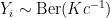 . For any prior on c with support on
  , the posterior given $Y$ converges to c.
A-há! Thanks for the link! The above is what I meant to write.
Rafael, I should also have reposted this reference, which describes our experiences in trying to implement various schemes, including the Gelfand-Dey idea.
Forgot to put the reference in!
Click to access 241.pdf
Similarly, here is a study of those computational techniques for evidence approximation:
I don’t think that we can talk about doing statistical inference for , at least not in a conventional sense. If we consider the simulated values of
  to be our “data”, then we need a likelihood
  , but
, but . This means that the sample “as it is” doesn’t bring any information about
  (I’m not writing
  or
or  because I’m adopting Larry’s point of view, so we are interested in the posterior
  ).
).
there no connection between the raw simulated values and the normalizing constant, hence
So the raw sample cannot be used to do inference about the constant. Then as Larry said, if you decide to use the sample to calculate density estimate of
  , you can use the estimator
  . Maybe we could call this a frequentist estimator, because it depends only on the sample, but we still have no probabilistic model connecting the sample to the constant.
For me the only way of constructing such a model is choosing an estimator of , and consider it to be your data. So maybe a (very stretched!) way of doing something that resambles Bayesian inference on this problem is:
 ) estimator of
  based on a sample
  , and call it
  .
. of the estimator under repeated Monte Carlo sampling from $P(\theta|Y)$.
 use
use  as your data,
  as your likelihood and then given a prior on $c$ you have something that looks like a posterior (up to another proportionality constant!).
\begin{enumerate}
\item choose an unbiased (
\item calculate (an approximation to) its finite sample distribution
\item given a sample
\end{enumerate}
Honestly, apart from all this procedure being quite crazy, I don’t think that we could say that is a proper likelihood
  . On the other hand if, after calculating
  we meet somebody who is unaware of what we have been doing, and we tell him “look:
  (for example) and this your prior
  , could you please give me a posterior for c”, then from the point of view of this person everything looks fine and stricly speaking we are not lying him.
The apparent paradox comes, I think, from the imprecise meaning attached to the assumption that “ is known”. From the point of view of Bayesian Numerical Analysis (as, e.g., in the book “Average-Case Analysis of Numerical Problems” by Klaus Ritter or in the older paper “Bayesian numerical analysis” by Persi Diaconis), it would be safer to say that
  is actually unknown, but that we are able to get information about it through some “actions” (if you prefer a decision-theoretic flavour) or “experiments” (if you prefer a more statistical flavour) that can be
a) either pointwise evaluations, i.e., the possibility to get at any
  ,
,
b) or the generation of samples from
from  .
.
To make sense of this problem, we have to acknowledge that there is a cost in getting information about through either a) or b). In the everyday statistician’s langage, “
 is known” typically means that pointwise evaluations are cheap (e.g., we have an analytical expression for it).
The focus in Larry’s post is on estimating using samples
  , …,
, …,  . However, note that
  is not identifiable if we can only sample from
  . Therefore, samples from
  must be used in combination with (at least one) pointwise evaluations of
  .
.
My “BNA” solution to this paradox would be as follows:
1) Choose a prior distribution on the function . I would typically assume a Gaussian process prior on
  .
.
2) This prior, together with the data ( , …,
, …,  and some pointwise evaluations of
  ), define as usual, through Bayes’ formula, a posterior distribution for the process
  (not a Gaussian process anymore, under the posterior).
3) This posterior induce a posterior for , where
  .
.
Formally this is it, but then come the practical considerations :
A) How to sample from the posterior of ? One possibility would be write a quadrature formula for
  (i.e., discretize the mapping
  ) and then to use the “swap” sampler proposed by Adams, Murray and MacKay (http://arxiv.org/abs/0912.4896) to sample the values of
  that are involved in this quadrature.
B) From a computational point of view, using such a fully Bayesian approach is only relevant if the cost for getting information about (through sampling or pointwise evaluations) is very high…
I hope this helps…
Ooops, I just saw that my approach is discussed in #4 of the initial post and deemed “unsatisfactory”…
Anyway, I still think that this is the only reasonable way of looking at this as a “statistical” problem (amenable to a Bayesian analysis).
Indeed, if you assume that is known in the usual statistical sense, then you have a “degenerate” statistical model with only one probability measure instead of a family, and there is nothing left to estimate (in other words,
  is a valid estimator under this model).
Even though knowing g(theta) in principle fixes c, the only way of knowing c involves solving a problem that is either too difficult or impossible to solve so that a direct solution is either infeasible or impossible. Although in principle c is a single value, identifying c is probably an ill-posed problem so that even direct approaches of solving the “inverse” problem (e.g. the harmonic mean) will fail spectacularly. Having said that, I believe there is a statistical problem to be solved by Bayesian means here, although the particulars of the problem create a framing effect that is blocking us from seeing this clearly.
For example, if one had a way to check a given value of c with its respect to its compatibility with the contraint imposed by c (as a symbol) being a normalization constant, then one could check one after one all possible values of c and find those that are most compatible with the normalization constraint. To bring the statistical problem out of the closet, we need to map the “check a given value of c with its respect to its compatibility with the constraint” to a likelihood function, and have some sort of prior belief on the various possible values of c (i.e. before carrying out the compatibility check), so that after performing the compatibility check we can update our belief into the posterior distribution of c. IMHO, the density estimation is the most fruitful starting point for recasting the problem into something that can be “solved” by statistical means while avoiding numerical integration (other than the one carried out by the MCMC method which gave us the posterior samples). So what could a possible Bayesian solution look like?
1) approximate the posterior density with a tractable, multivariate approximation (e.g. a Dirichlet Process mixture of smooth densities estimated by MCMC if it can work in the highdimensional spaces we are contemplating or a GP if this works any better) based on the samples generated by the MCMC run that evaluated . Call this density estimate
 covering the “interesting” (to the eyes of the beholder) areas of the posterior density, sample the value of
  from whatever Bayesian density estimator was used in the first step
 and the (known)
  playing the role of an offset in linear model vernacular. The intercept in this regression model corresponds to the sought after normalization constant
2) for a sequence of theta
3) set up a bona fide linear regression between
4) summarize the posterior density for the normalization constant using conventional summaries and select the point estimator implied by one’s favorite loss function
I’m sure there are holes to be poked in this solution, but at least it avoids frequentist estimators for the density step, fully acknowledging the uncertainty implicit in the density estimation step for the value for the (step 2). As far as I can tell, it is a fully conditional approach, since conditions on both the posterior samples from the density whose normalization constant we try to compute (step 1) and the relationship between this density and
  (step 3).
This seems like precisely the problem of ‘logical uncertainty’: how formally deal with uncertainty about what things are implied by assumptions.
A solution to this problem would be *really* valuable in AI, but it is a pretty hard problem. Lots of people have devoted lots of time to it and haven’t gotten far.
I made it to this page and the one on stack exchange when I try to find solutions for my problem. What I need is to compute the marginal likelihood and that is exactly c : (correct me if i’m wrong). So one of the solutions that I found is to use Laplace-Metropolis approximation
  where d is the size of
  is the mode of f and A is minus inverse of hessian matrix of f at
  . In that way, we can see $\latex f = log(L(\theta)\pi(\theta)$ and we can get use of data to estimate c.
Sorry about the typo, but once posted the comment I don’t know how to adit the post.
 where d is the size of
  is where f attains its maximum and A is minus inverse of hessian matrix of f at
  .
. we can get use of data to estimate c
I rewrite the formula in this reply :
marginal likelihood =
By posing
I arrive in the discussion a bit late! But since nobody seems to have mentioned it yet, I’d like to mention Sequential Monte Carlo samplers. In your presentation of the problem, you already have a sample from the posterior, e.g. from a MCMC chain. However if you already know that you’re interested in the normalizing constant before sampling, then it might be better to use something else than MCMC. SMC samplers provide an estimate of the normalizing constant as a by product of posterior approximation, see e.g. Doucet Del Moral Jasra 2006 (http://www.stats.ox.ac.uk/~doucet/delmoral_doucet_jasra_sequentialmontecarlosamplersJRSSB.pdf), Schweizer 2012 (http://arxiv.org/pdf/1204.2382.pdf), Whiteley 2012 (http://www.maths.bris.ac.uk/~manpw/SAP-Whiteley-FINAL-031312.pdf) for some recent theoretical validation.
The normalizing constant estimate from SMC sampler is unbiased, has a variance decreasing linearly with the number N of particles, increasing linearly with the number T of data points in a Bayesian setting (so that taking N as a linear function of T, you can control it uniformly), and polynomial in the dimension (see Schweizer 2012). This holds under some conditions of course, but it’s already better than the MCMC-based approaches for the normalizing constant.
An direct application to model choice is proposed in Zhou, Johansen, Aston 2013: http://arxiv.org/abs/1303.3123
To summarize, instead of trying to take the output of an MCMC chain and figure out how to estimate the constant from that, there are also other Monte Carlo methods that can be considered. SMC samplers might soon become the standard tools for this.
Actually I did mention it. But that’s OK. MC sampling already is the standard tool in geophysical inverse theory. Has been for many years.
Fail to see where you did. I’d be very interested in any reference to the use of Sequential Monte Carlo samplers in geophysics.
Google sequential Monte Carlo geophysics. Also Google Monte Carlo geophysics. The latter will pick up a nice historical review by Mosegaard and Sambridge. The former will give you lots of current research articles.
Found some use of particle filters, which in state space models provide approximations of L(theta) for a given theta, in Larry’s notation. Couldn’t find a reference to SMC samplers approximating the constant c. Any reference?
One Trackback
[…] https://normaldeviate.wordpress.com/2012/10/05/the-normalizing-constant-paradox/ Share this:TwitterMorePrintLinkedInDiggFacebookEmailLike this:LikeBe the first to like this. […]