Steve Marron on “Big Data”

Steve Marron is a statistician at UNC. In his younger days he was well known for his work on nonparametric theory. These days he works on a number of interesting things including analysis of structured objects (like tree-structured data) and high dimensional theory.

Steve sent me a thoughtful email the other day about “Big Data” and, with his permission, I am posting it here.

I agree with pretty much everything he says. I especially like these two gems: First, “a better funded statistical community would be a more efficient way to get such things done without all this highly funded re-discovery.” And second: “I can see a strong reason why it DOES NOT make sense to fund our community better. That is our community wide aversion to new ideas.”

Enough from me. Here is Steve’s comment:

Guest Post, by Steve Marron

My colleagues and I have lately been discussing “Big Data”, and your blog was mentioned.

Not surprisingly you’ve got some interesting ideas there. Here come some of my own thoughts on the matter.

First should one be pessimistic? I am not so sure. For me exhibit A is my own colleagues. When such things came up in the past (and I believe that this HAS happened, see the discussion below) my (at that time senior) colleagues were rather arrogantly ignorant. Issues such as you are raising were blatantly pooh poohed, if they were ever considered at all. However, this time around, I am seeing a far more different picture. My now mostly junior colleagues are taking this very seriously, and we are currently engaged in major discussion as to what we are going to do about this in very concrete terms such as course offerings, etc. In addition, while some of my colleagues think in terms of labels such as “applied statistician”, “theoretical statistician” and “probabilist”, everybody across the board is jumping in. Perhaps this is largely driven by an understanding that universities themselves are in a massive state of flux, and that one had better be a player, or else be totally left behind. But it sure looks better than some of the attitudes I saw earlier on in my career.

Now about the bigger picture. I think there is an important history here that you are totally ignoring. In particular, I view “Big Data” as just the latest manifestation of a cycle that has been rolling along for quite a long time. Actually I have been predicting the advent of something of this type for quite a while (although I could not predict the name, nor the central idea).

Here comes a personally slanted (certainly over-simplified) view of what I mean here. Think back on the following set of “exciting breakthroughs”:

– Statistical Pattern Recognition
– Artificial Intelligence
– Neural Nets
– Data Mining
– Machine Learning

Each of these was started up in EE/CS. Each was the fashionable hot topic (considered very sexy and fresh by funding agencies) of its day. Each was initially based on usually one really cool new idea, which was usually far outside of what folks working in conventional statistics had any hope (well certainly no encouragement from the statistical community) of dreaming up. I think each attracted much more NSF funding than all of statistics ever did, at any given time. A large share of the funding was used for re-invention of ideas that already existed in statistics (but would get a sexy new name). As each new field matured, there came a recognition that in fact much was to be gained by studying connections to statistics, so there was then lots of work “creating connections”.

Now given the timing of these, and how they each have played out, over time, it had been clear to me for some time that we were ripe for the next one. So the current advent of Big Data is no surprise at all. Frankly I am a little disappointed that there does not seem to be any really compelling new idea (e.g. as in neural nets or the kernel embedding idea that drove machine learning). But I suspect that the need for such a thing to happen to keep this community properly funded has overcome the need for an exciting new idea. Instead of new methodology, this seems to be more driven by parallelism and cloud computing. Also I seem to see larger applied math buy-in than there ever was in the past. Maybe this is the new parallel to how optimization has appeared in a major way in machine learning.

Next, what should we do about it? Number one of course is to get engaged, and as noted above, I am heartened at least at my own local level as discussed above.

I generally agree with your comment about funding, and I can think of ways to sell statistics. For example, we should make the above history clear to funding agencies, and point out that in each case there has been a huge waste of resources on people doing a large amount of rediscovery. In most of those areas, by the time the big funding hits, the main ideas are already developed so the funding really just keeps lots of journeymen doing lots of very low impact work, with large amounts of rediscovery of things already known in the statistical community. The sell could be that a better funded statistical community would be a more efficient way to get such things done without all on this highly funded re-discovery.

But before making such a case, I suggest that is it important to face up to our own shortcomings, from the perspective of funding agencies. I can see a strong reason why it DOES NOT make sense to fund our community better. That is our community wide aversion to new ideas. While I love working with statistical concepts, and have a personal love of new ideas, it has not escaped my notice that I have always been in something of a minority in that regard. We not only do not choose to reward creativity, we often tend to squelch it. I still remember the first time I applied for an NSF grant. I was ambitious, and the reviews I got back said the problem was interesting, but I had no track record, the reviewers were skeptical of me, and I did not get funded. This was especially frustrating as by the time I got those reviews I had solved the stated problem. It would be great if that could be regarded as an anomaly of the past when folks may have been less enlightened than now. However, I have direct evidence that this is not true. Unfortunately exactly that cycle repeated itself for one of my former students on this very last NSF cycle.

What should we do to deserve more funding? Somehow we need a bigger tent, which is big enough to include the creative folks who will be coming up with the next really big ideas (big enough to include the folks who are going to spawn the next new community, such as those listed above). This is where research funding should really be going to be most effective.

Maybe more important, we need to find a way to create a statistical culture that reveres new ideas, instead of fearing and shunning them.

Best, Steve

Brad Efron, Tornadoes, and Diane Sawyer

Brad Efron wrote to me and posed an interesting statistical question:

“Last Wednesday Diane Sawyer interviewed an Oklahoma woman who twice
had had her home destroyed by a force-4 tornado. “A one in a
hundred-trillion chance!” said Diane. ABC showed a nice map with the
current storm’s track of destruction shaded in, about 18 miles long
and 1 mile wide. Then the track of the 1999 storm was superimposed,
about the same dimensions, the two intersecting in a roughly 1 square
mile lozenge. Diane added that the woman “lives right in the center of
Tornado alley.”

Question: what odds should have Diane quoted? (and for that matter,
what is the right event to consider?)

Regards, Brad”

Anyone have a good answer?

By the way, I should add that Diane Sawyer has a history of
broadcasting stories filled with numerical illiteracy. She did a long
series opposing the use of lean finely textured beef (LFTB), also
known as “pink slime.” In fact, LFTB is perfectly healthy, its use
requires slaughtering many fewer cows each year and makes meat cheaper
for poor people. The series was denounced by many scientists and even
environmentalists. ABC is being sued for over one billion dollars.

She also did a long series on “Buy America” encouraging people to
shun cheap goods from abroad. This is like telling people who live in
Cleveland to shun buying any products and services not produced in
Cleveland (including not watching ABC news which is produced in New
York, or reading statistics papers not written in Cleveland.) This
high-school level mistake in economics is another example of Ms.
Sawyer’s numerical illiteracy.

But I digress.

Let’s return to Brad’s question:

What is a good way to compute the odds that someone has their house
destroyed by a tornado twice?

I open it up for discussion.

STEIN’S PARADOX

STEIN’S PARADOX

Something that is well known in the statistics world but perhaps less well known in the machine learning world is Stein’s paradox.

When I was growing up, people used to say: do you remember where you were when you heard that JFK died? (I was three, so I don’t remember. My first memory is watching the Beatles on Ed Sullivan.)

Similarly, statisticians used to say: do you remember where you were when you heard about Stein’s paradox? That’s how surprising it was. (I don’t remember since I wasn’t born yet.)

Here is the paradox. Let . Define the risk of an estimator to be

An estimator is inadmissible if there is another estimator with smaller risk. In other words, if

with strict inequality at at least one .

Question: Is admissible.
Answer: Yes.

Now suppose that where now , and

Question: Is admissible.
Answer: Yes.

Now suppose that where now , and

Question: is admissible.
Answer: No!

If you don’t find this surprising then either you’ve heard this before or you’re not thinking hard enough. Keep in mind that the coordinates of the vector are independent. And the could have nothing to do with each other. For example, mass of the moon, price of coffee and temperature in Rome.

In general, is inadmissible if the dimension of satisfies .

The proof that is inadmissible is based on defining an explicit estimator that has smaller risk than . For example, the James-Stein estimator is

It can be show that the risk of this estimator is strictly smaller than the risk of , for all . This implies that is inadmissible. If you want to see the detailed calculations, have a look at Iain Johnstone’s at this site which he makes freely available on his website.

Note that the James-Stein estimator shrinks towards the origin. (In fact, you can shrink towards any point; there is nothing special about the origin.) This can be viewed as an empirical Bayes estimator where has a prior of the form and is estimated from the data. The Bayes explanation gives some nice intuition. But it’s also a bit misleading. The Bayes explanation suggests we are shrinking the means together because we expect them a priori to be similar. But the paradox holds even when the means are not related in any way.

Some intuition can be gained by thinking about function estimation. Consider a smooth function . Suppose we have data

where and . Let us expand in an orthonormal basis: 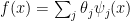. To estimate we need only estimate the coefficients . Note that . This suggests the estimator

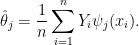
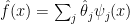But the resulting function estimator is useless because it is too wiggly. The solution is to smooth the estimator; this corresponds to shrinking the raw estimates towards 0. This adds bias but reduces variance. In other words, the familiar process of smoothing, which we use all the time for function estimation, can be seen as “shrinking estimates towards 0” as with the James-Stein estimator.

If you are familiar with minimax theory, you might find the Stein paradox a bit confusing. The estimator is minimax, that is, it’s risk achieves the minimax bound

This suggests that is a good estimator. But Stein’s paradox tells us that is inadmissible which suggests that it is a bad estimator.

Is there a contradiction here?

No. The risk of is a constant. In fact, for all where is the dimension of . The risk of the James-Stein estimator is less than the risk of , but, as . So they have the same maximum risk.

On the one hand, this tells us that a minimax estimator can be inadmissible. On the other hand, in some sense it can’t be “too far” from admissible since they have the same maximum risk.

Stein first reported the paradox in 1956. I suspect that fewer and fewer people include the Stein paradox in their teaching. (I’m guilty.) This is a shame. Paradoxes really grab students’ attention. And, in this case, the paradox is really fundamental to many things including shrinkage estimators, hierarchical Bayes, and function estimation.

Aaronson, COLT, Bayesians and Frequentists

Aaronson, COLT, Bayesians and Frequentists

I am reading Scott Aaronson’s book “Quantum Computing Since Democritus” which can be found here.

The book is about computational complexity, quantum mechanics, quantum computing and many other things. It’s a great book and I highly recommend it. Much of the material on complexity classes is tough going but you can skim over some of the details and still enjoy the book. (That’s what I am doing.) There at least 495 different complexity classes: see the complexity zoo. I don’t know how anyone can keep track of this.

Anyway, there is a chapter on computational learning theory that I wanted to comment on. (There is another chapter about probabilistic reasoning and the anthropic principle which I’ll comment on in a future post.) Scott gives a clear introduction to learning theory and he correctly traces the birth of the theory to Leslie Valiant’s 1984 paper that introduced PAC (probably almost correct) learning. He also contrasts PAC learning with Bayesian learning.

Now I want to put on my statistical curmudgeon hat and complain about computational learning theory. My complaint is this: the discovery of computational learning theory is nothing but the re-discovery of a 100 year old statistical idea called a “confidence interval.”

Let’s review some basic learning theory. Let denote all axis aligned rectangles in the plane. We can think of each rectangle as a classifier: predict if and predict if . Suppose we have data . If we pick the rectangle that makes the fewest classification errors on the data, will we predict well on a new observation? More formally: is the empirical risk estimator a good predictor?

Yes. The reason is simple. Let be the prediction risk and let

be the empirical estimate of the risk. We would like to claim that is close to the best classifier in . That is, we would like to show that is close to , with high probability. This fact follows easily if we can show that

is small with high probability. And this does hold since the VC dimension of is finite. Specifically, the key fact is that, for any distribution of the data , we have

for known constants and .

But this is equivalent to saying that a confidence interval for is

where

That is, for any distribution ,

As Scott points out, what distinguishes this type of reasoning from Bayesian reasoning, is that we require this to hold uniformly, and that there are no priors involved. To quote from his book:

This goes against a belief in the Bayesian religion, that if your priors are different then you come to an entirely different conclusion. The Bayesian starts out with a probability distribution over the possible hypotheses. As you get more and more data, you update this distribution using Bayes’s rule.

That’s one way to do it, but computational learning theory tells us that it’s not the only way. You don’t need to start out with any assumptions about a probability distribution over the hypotheses … you’d like to learn any hypothesis in the concept class, for any sample distribution, with high probability over the choice of samples. In other words, you can trade the Bayesians’ probability distribution over hypotheses for a probability distribution over sample data.

(Note: “hypothesis” = classifier and “concept class” = set of classifiers, “learn” = estimate).

Now, I agree completely with the above quote. But as I said, it is basically the definition of a frequentist confidence interval.

So my claim is that computational learning theory is just the application of frequentist confidence intervals to classification.

There is nothing bad about that. The people who first developed learning theory were probably not aware of existing statistical theory so they re-developed it themselves and they did it right.

But it’s my sense — and correct me if I’m wrong — that many people in computational learning theory are still woefully ignorant about the field of statistics. It would be nice if someone in the field read the statistics literature and said: “Hey, these statistics guys did this 50 years ago!”

Am I being too harsh?