Stein’s Method

I have mentioned Stein’s method in passing, a few times on this blog. Today I want to talk about Stein’s method in a bit of detail.

1. What Is Stein’s Method?

Stein’s method, due to Charles Stein, is actually quite old, going back to 1972. But there has been a great deal of interest in the method lately. As in many things, Stein was ahead of his time.

Stein’s method is actually a collection of methods for showing that the distribution ${F_n}$ of some random variable ${X_n}$ is close to Normal. What makes Stein’s method so powerful is that it can be used in a variety of situations (including cases with dependence) and it tells you how far ${F_n}$ is from Normal.

I will follow Chen, Goldstein and Shao (2011) quite closely.

2. The Idea

Let ${X_1,\ldots, X_n\in \mathbb{R}}$ be iid with mean 0 and variance 1. Let

$\displaystyle X = \sqrt{n}\ \overline{X}_n =\frac{1}{\sqrt{n}}\sum_i X_i$

and let ${Z\sim N(0,1)}$ . We want to bound

$\displaystyle \Delta_n = \sup_z \Bigl| \mathbb{P}(X \leq z) - \mathbb{P}( Z \leq z)\Bigr| = \sup_z \Bigl| \mathbb{P}(X \leq z) - \Phi(z)\Bigr|$

where ${\Phi}$ is the cdf of a standard Normal. For simplicity, we will assume here

$\displaystyle |X_i| \leq B < \infty$

but this is not needed. The key idea is this:

$\displaystyle \mathbb{E}[Y f(Y)] = \mathbb{E}[f'(Y)]$

for all smooth ${f}$ if and only if ${Y\sim N(0,1)}$ . This suggests the following idea: if we can show that ${\mathbb{E}[Y f(Y)-f'(Y)]}$ is close to 0, then ${Y}$ should be almost Normal.

More precisely, let ${Z\sim N(0,1)}$ and let ${h}$ be any function such that ${\mathbb{E}|h(Z)| < \infty}$ . The Stein function ${f}$ associated with ${h}$ is a function satisfying

$\displaystyle f'(x) - x f(x) = h(x) - \mathbb{E}[h(Z)].$

It then follows that

$\displaystyle \mathbb{E}[h(X)] - \mathbb{E}[h(Z)]= \mathbb{E}[f'(X) - Xf(X)]$

and showing that ${X}$ is close to normal amounts to showing that ${\mathbb{E}[f'(X) - Xf(X)]}$ is small.

Is there such an ${f}$ ? In fact, letting ${\mu = \mathbb{E}[h(Z)]}$ , the Stein function is

$\displaystyle f(x) =f_h(x)= e^{x^2/2}\int_{-\infty}^x[ h(y) - \mu] e^{-y^2/2} dy. \ \ \ \ \ (1)$

More precisely, ${f_h}$ is the unique solution to the above equation subject to the side condition ${\lim_{x\rightarrow\pm\infty} e^{-x^2/2}f(x) = 0}$ .

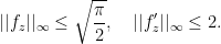
Let’s be more specific. Choose any ${z\in \mathbb{R}}$ and let ${h(x) = I(x\leq z) - \Phi(z)}$ . Let ${f_z}$ denote the Stein function for ${h}$ ; thus ${f_z}$ satisfies

$\displaystyle f_z'(x)-xf_z(x) = I(x\leq z) - \Phi(z).$

The unique bounded solution to this equation is

$\displaystyle f(x)\equiv f_z(x) = \begin{cases} \sqrt{2\pi}e^{x^2/2}\Phi(x)[1-\Phi(z)] & x\leq z\\ \sqrt{2\pi}e^{x^2/2}\Phi(z)[1-\Phi(x)] & x> z. \end{cases}$

The function ${f_z}$ has the following properties:

$\displaystyle \Bigl| (x+a)f_z(x+a) - (x+b)f_z(x+b) \Bigr| \leq ( |x| + c)(|a|+|b|)$

where ${c = \sqrt{2\pi}/4}$ . Also,

$\displaystyle ||f_z||_\infty \leq \sqrt{\frac{\pi}{2}},\ \ \ ||f'_z||_\infty \leq 2.$

Let ${{\cal F} = \{f_z:\ z\in \mathbb{R}\}}$ . From the equation ${f'(x) - x f(x) = h(x) - \mathbb{E}[h(Z)]}$ it follows that

$\displaystyle \mathbb{P}(X \leq z) - \mathbb{P}(Y \leq z) = \mathbb{E}[f'(X) - Xf(X)]$

and so

$\displaystyle \Delta_n = \sup_z \Bigl| \mathbb{P}(X \leq z) - \mathbb{P}( Z \leq z)\Bigr| \leq \sup_{f\in {\cal F}} \Bigl| \mathbb{E}[ f'(X) - X f(X)]\Bigr|.$

We have reduced the problem of bounding ${\sup_z \Bigl| \mathbb{P}(X \leq z) - \mathbb{P}( Z \leq z)\Bigr|}$ to the problem of bounding 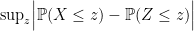${\sup_{f\in {\cal F}} \Bigl| \mathbb{E}[ f'(X) - X f(X)]\Bigr|}$ .

3. Zero Bias Coupling

As I said, Stein’s method is really a collection of methods. One of the easiest to explain is “zero-bias coupling.”

Let ${\mu_3 = \mathbb{E}[|X_i|^3]}$ . Recall that ${X_1,\ldots,X_n}$ are iid, mean 0, variance 1. Let

$\displaystyle X = \sqrt{n}\ \overline{X}_n = \frac{1}{\sqrt{n}}\sum_i X_i = \sum_i \xi_i$

where

$\displaystyle \xi_i = \frac{1}{\sqrt{n}} X_i.$

For each ${i}$ define the leave-one-out quantity

$\displaystyle X^i = X - \xi_i$

which plays a crucial role. Note that ${X^i}$ is independent of ${X_i}$ . We also make use of the following simple fact: for any ${y}$ and ${a}$ , ${\Phi(y+a) - \Phi(y)\leq a/\sqrt{2\pi}}$ since the density of the Normal is bounded above by ${1/\sqrt{2\pi}}$ .

Recall that ${X\sim N(0,\sigma^2)}$ if and only if

$\displaystyle \sigma^2 \mathbb{E}[f'(X)] = \mathbb{E}[X f(X)]$

for all absolutely continuous functions ${f}$ (for which the expectations exists). Inspired by this, Goldstein and Reinert (1997) introduced the following definition. Let ${X}$ be any mean 0 random variable with variance ${\sigma^2}$ . Say that ${X^*}$ has the ${X}$ -zero bias distribution if

$\displaystyle \sigma^2 \mathbb{E} [f'(X^*)] = \mathbb{E}[X f(X)].$

for all absolutely continuous functions ${f}$ for which ${\mathbb{E}| X f(X)|< \infty}$ . Zero-biasing is a transform that maps one random variable ${X}$ into another random variable ${X^*}$ . (More precisely, it maps the distribution of ${X}$ into the distribution of ${X^*}$ .) The Normal is the fixed point of this map. The following result shows that ${X^*}$ exists and is unique.

Theorem 1 Let ${X}$ be any mean 0 random variable with variance ${\sigma^2}$ . There exists a unique distribution corresponding to a random variable ${X^*}$ such that

$\displaystyle \sigma^2 \mathbb{E}[f'(X^*)] = \mathbb{E}[X f(X)]. \ \ \ \ \ (2)$

for all absolutely continuous functions ${f}$ for which ${\mathbb{E}| X f(X)|< \infty}$ . The distribution of ${X^*}$ has density

$\displaystyle p^*(x) = \frac{\mathbb{E}[ X I(X>x)]}{\sigma^2} = -\frac{\mathbb{E}[ X I(X\leq x)]}{\sigma^2}.$

Proof: It may be verified that ${p^*(x) \geq 0}$ and integrates to 1. Let us verify that (2) holds. For simplicity, assume that ${\sigma^2=1}$ . Given an absolutely continuous ${f}$ there is a ${g}$ such that ${f(x) = \int_0^x g}$ . Then

$\displaystyle \begin{array}{rcl} \int_0^\infty f'(u)\ p^*(u) du &=& \int_0^\infty f'(u)\ \mathbb{E}[X I(X>u)] du = \int_0^\infty g(u)\ \mathbb{E}[X I(X>u)] du\\ &=& \mathbb{E}\left[X \int_0^\infty g(u) I(X>u) du \right]= \mathbb{E}\left[X \int_{0}^{X\vee 0} g(u) du \right]= \mathbb{E}[X f(X)I(X\geq 0)]. \end{array}$

Similarly, ${\int_{-\infty}^0 f'(u)\ p^*(u) du =\mathbb{E}[X f(X)I(X\geq 0)].}$ $\Box$

Here is a way to construct ${X^*}$ explicitly when dealing with a sum.

Lemma 2 Let ${\xi_1,\ldots, \xi_n}$ be independent, mean 0 random variables and let ${\sigma_i^2 = {\rm Var}(\xi_i)}$ . Let ${W =\sum_i \xi_i}$ . Let ${\xi_1^*,\ldots, \xi_n^*}$ be independent and zero-bias. Define

$\displaystyle W^* = W - \xi_J + \xi_J^*$

where ${\mathbb{P}(J=i)=\sigma_i^2}$ . Then ${W^*}$ has the ${W}$ -zero bias distribution. In particular, suppose that ${X_1,\ldots, X_n}$ have mean 0 common variance and let ${W = \frac{1}{\sqrt{n}}\sum_i X_i}$ . Let ${J}$ be a random integer from 1 to ${n}$ . Then ${W^* = W - \frac{1}{\sqrt{n}}X_J + \frac{1}{\sqrt{n}}X_J^*}$ has the ${W}$ -zero bias distribution.

Now we can prove a Central Limit Theorem using zero-biasing.

Theorem 3 Suppose that ${|X_i| \leq B}$ . Let ${Y\sim N(0,1)}$ . Then

$\displaystyle \sup_z \Bigl| \mathbb{P}(X \leq z) - \mathbb{P}( Y \leq z)\Bigr| \leq \frac{6 B}{\sqrt{n}}.$

Proof: Let ${X_1^*,\ldots, X_n^*}$ be independent random variables where ${X_i^*}$ is zero-bias for ${X_i}$ . Let ${J}$ be chosen randomly from ${\{1,\ldots, n\}}$ and let

$\displaystyle X^* = X - \frac{1}{\sqrt{n}}(X_J - X_J^*).$

Then, by the last lemma, ${X^*}$ is zero-bias for ${X}$ and hence

$\displaystyle \mathbb{E}[ X f(X)] = \mathbb{E}[f'(X^*)] \ \ \ \ \ (3)$

for all absolutely continuous ${f}$ . Also note that

$\displaystyle |X^* - X| \leq \frac{2B}{\sqrt{n}} \equiv \delta. \ \ \ \ \ (4)$

So,

$\displaystyle \begin{array}{rcl} \mathbb{P}(X \leq z) - \mathbb{P}(Y \leq z) &\leq & \mathbb{P}(X \leq z) - \mathbb{P}(Y \leq z+\delta) +\mathbb{P}(Y \leq z+\delta) -\mathbb{P}(Y \leq z) \leq \mathbb{P}(X \leq z) - \mathbb{P}(Y \leq z+\delta) + \frac{\delta}{\sqrt{2\pi}}\\ &\leq & \mathbb{P}(X^* \leq z+\delta) - \mathbb{P}(Y \leq z+\delta) + \frac{\delta}{\sqrt{2\pi}} \leq \sup_z |\mathbb{P}(X^* \leq z+\delta) - \mathbb{P}(Y \leq z+\delta)| + \frac{\delta}{\sqrt{2\pi}}\\ &=& \sup_z |\mathbb{P}(X^* \leq z) - \mathbb{P}(Y \leq z)| + \frac{\delta}{\sqrt{2\pi}}. \end{array}$

By a symmetric argument, we deduce that

$\displaystyle \sup_z |\mathbb{P}(X \leq z) - \mathbb{P}(Y \leq z)| \leq \sup_z |\mathbb{P}(X^* \leq z) - \mathbb{P}(Y \leq z)| + \frac{\delta}{\sqrt{2\pi}}.$

Let ${f=f_z}$ . From the properties of the Stein function given earlier we have

$\displaystyle \begin{array}{rcl} \sup_z |\mathbb{P}(X^* \leq z) - \mathbb{P}(Y \leq z)| &\leq & \sup_{f\in {\cal F}}\Big|\mathbb{E}[ f'(X^*) - X^* f(X^*)]\Bigr|= \sup_{f\in {\cal F}}\Big|\mathbb{E}[ X f(X) - X^* f(X^*)]\Bigr|\\ &\leq & \mathbb{E}\left[ \left( |X| + \frac{2\pi}{4}\right)\ |X^* - X| \right]\leq \delta \left(1 + \frac{2\pi}{4}\right). \end{array}$

Combining these inequalities we have

$\displaystyle \sup_z |\mathbb{P}(X \leq z) - \mathbb{P}(Y \leq z)| \leq \delta \left(1 + \frac{1}{\sqrt{2\pi}} + \frac{2\pi}{4}\right)\leq 3\delta =\frac{6 B}{\sqrt{n}}.$

$\Box$

4. Conclusion

This is just the tip of the iceberg. If you want to know more about Stein’s method, see the references below. I hope I have given you a brief hint of what it is all about.

References

Chen, Goldstein and Shao. (2011). Normal Approximation by Stein’s Method. Springer.

Nourdin and Peccati (2012). Normal Approximations With Malliavin Calculus. Cambridge.

Ross, N. (2011). Fundamentals of Stein’s method . Probability Surveys, 210-293. link

10 Comments

Twan van Laarhoven

Posted November 16, 2013 at 7:28 pm | Permalink

The wikipedia link at the start of the article is missing an apostrophe, it should link to http://en.wikipedia.org/wiki/Stein%27s_method

I don’t understand the start of section 3. You say that \xi_i = 1/\sqrt{n} X_i and X^i = X_i-\xi_i. So X^i = (1-1/\sqrt{n}) X_i, which is most certainly not independent of X_i. Did you mean X^i = X – \xi_i?
- normaldeviate
  
  Posted November 16, 2013 at 7:38 pm | Permalink
  
  yes on both
  i made the corrections
  thanks
Bill Jefferys

Posted November 16, 2013 at 7:35 pm | Permalink

Larry: Something weird has happened to the LaTeX near the end of the article. The aspect ratio of the characters is screwed up making the formulas hard to read.
- normaldeviate
  
  Posted November 16, 2013 at 7:40 pm | Permalink
  
  It looks fine in my browser.
  Maybe it is browser dependent?
coreyyanofsky

Posted November 19, 2013 at 8:04 am | Permalink

My intuition says that one could use Stein’s method to check on the closeness of a RV’s distribution to *any* other distribution, not just Normal, as follows: Suppose we want to check if a random variable X’ has a distribution close to F. Define Z’ as a random variable with distribution F and quantile function q; then Z = Psi(q(Z’)) has a Normal distribution. Does it not follow that X’ will have distribution close to F if X = Psi(q(X’)) has a distribution close to Normal?
- coreyyanofsky
  
  Posted November 19, 2013 at 8:11 am | Permalink
  
  Whoops, I think I got the bijection backwards: it should be Z = q(F(Z’)), where q is now the quantile function of the Normal distribution.
- normaldeviate
  
  Posted November 19, 2013 at 8:14 am | Permalink
  
  Yes Stein’s method extends to other distributions too.
  One has to develop the correct differential equation.
  There is a chapter on this in the Chen, Goldstein, Shao book.
Edward

Posted December 5, 2013 at 8:27 pm | Permalink

The Wikipedia page for Stein’s method mentions that it can be used to prove the central limit theorem – does it have any other particularly useful applications?
- normaldeviate
  
  Posted December 5, 2013 at 8:29 pm | Permalink
  
  It is used to prove that the distribution of some random variable X_n
  is close to its limiting distribution.
  Normal is a special case.
ashish soni

Posted February 18, 2014 at 2:29 am | Permalink

To what other distributions the Stein’s method is applicable to?

3 Trackbacks

By Rtistry & Rbominations :: linklist, sunday 2013-11-17 on November 17, 2013 at 5:58 pm

[…] Stein’s Method […]
By Means and Markov’s Inequality | Eventually Almost Everywhere on December 28, 2013 at 4:22 pm

[…] Stein’s Method (normaldeviate.wordpress.com) […]
By Mixing of the Noisy Voter Model | Eventually Almost Everywhere on March 23, 2014 at 5:32 pm

[…] Stein’s Method […]

Normal Deviate

Stein’s Method

10 Comments

3 Trackbacks

Recent Posts

Archives

Categories

Meta

Follow Blog via Email

RSS

Blog Stats

Search

Blogroll

RSS Feeds

Meta

Normal Deviate

Stein’s Method

Share this:

Related

10 Comments

3 Trackbacks

Recent Posts

Archives

Categories

Meta

Follow Blog via Email

RSS

Blog Stats

Search

Blogroll

RSS Feeds

Meta