Robins and Wasserman Respond to a Nobel Prize Winner Continued: A Counterexample to Bayesian Inference?
This is a response to Chris Sims’ comments on our previous blog post. Because of the length of our response, we are making this a new post rather than putting it in the comments of the last post.
Recall that we observe 


Define ![{\theta \left( X\right) \equiv E \left[ Y|X\right]}](https://s0.wp.com/latex.php?latex=%7B%5Ctheta+%5Cleft%28+X%5Cright%29+%5Cequiv+E+%5Cleft%5B+Y%7CX%5Cright%5D%7D&bg=ffffff&fg=000000&s=0&c=20201002)
![{\pi \left( X\right) \equiv E\left[ R|X\right]}](https://s0.wp.com/latex.php?latex=%7B%5Cpi+%5Cleft%28+X%5Cright%29+%5Cequiv+E%5Cleft%5B+R%7CX%5Cright%5D%7D&bg=ffffff&fg=000000&s=0&c=20201002)

density 


![\displaystyle \psi \equiv E\left[ Y\right] =E\left\{ E\left[ Y|X\right] \right\} = E\left\{E\left[ Y|X,R=1\right] \right\} =\int_{[0,1]^d} \theta \left( x\right) dx.](https://s0.wp.com/latex.php?latex=%5Cdisplaystyle+++%5Cpsi+%5Cequiv+E%5Cleft%5B+Y%5Cright%5D+%3DE%5Cleft%5C%7B+E%5Cleft%5B+Y%7CX%5Cright%5D+%5Cright%5C%7D+%3D++E%5Cleft%5C%7BE%5Cleft%5B+Y%7CX%2CR%3D1%5Cright%5D+%5Cright%5C%7D+%3D%5Cint_%7B%5B0%2C1%5D%5Ed%7D+%5Ctheta+%5Cleft%28+x%5Cright%29+dx.++&bg=ffffff&fg=000000&s=0&c=20201002)
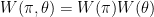
The likelihood

factors into two parts – the first depending on 

1. Selection Bias
This is a point of agreement. There is selection bias if and only if

Note that
![\displaystyle E\left[ Y\right] =E\left[ Y|R=1\right] - \frac{Cov\left\{ \theta \left(X\right) ,\pi \left( X\right) \right\} }{E[R]}.](https://s0.wp.com/latex.php?latex=%5Cdisplaystyle+++E%5Cleft%5B+Y%5Cright%5D+%3DE%5Cleft%5B+Y%7CR%3D1%5Cright%5D+-++%5Cfrac%7BCov%5Cleft%5C%7B+%5Ctheta+%5Cleft%28X%5Cright%29+%2C%5Cpi+%5Cleft%28+X%5Cright%29+%5Cright%5C%7D+%7D%7BE%5BR%5D%7D.++&bg=ffffff&fg=000000&s=0&c=20201002)
Hence, if 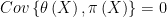
the sample average of
![\displaystyle \psi \equiv E\left[ Y\right] =\int_{[0,1]^d}\ \theta \left( x\right) dx.](https://s0.wp.com/latex.php?latex=%5Cdisplaystyle+++%5Cpsi+%5Cequiv+E%5Cleft%5B+Y%5Cright%5D+%3D%5Cint_%7B%5B0%2C1%5D%5Ed%7D%5C+%5Ctheta+%5Cleft%28+x%5Cright%29+dx.++&bg=ffffff&fg=000000&s=0&c=20201002)
In this case, inference is easy for the Bayesian and the frequentist and there is no issue. So we all agree that the interesting case is where there is selection bias,
that is, where

2. Posterior Dependence on 
If the prior 


We note that no one, Bayesian or frequentist, has ever proposed using an estimator that does not depend on 
3. Prior Independence Versus Selection Bias
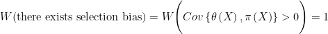
Reading Chris’ comments, the reader might get the impression that prior independence rules out selection bias, i.e. that is,

Therefore, one might conclude that if we want to discuss the interesting case where there is selection bias, then we cannot have 
But this is incorrect. 
Suppose that 


where 


Then, clearly 


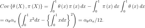
Hence
since 
4. Other Justifications For Prior Dependence?
Since prior independence of 
Suppose a new HMO needs to estimate the fraction 

by following 5000 of the 50,000 HMO members for a year. Because MI is a rare event, he oversampled subjects whose
smaller probability 

sampling fraction 

The world’s leading heart expert, our Bayesian, was hired to estimate 


As world’s expert, his beliefs about the risk function 


What’s more, Robins and Ritov (1997) showed that, if before seeing the data, any Bayesian, cardiac expert or not, thoroughly queries the epidemiologist
(who selected 


5. Alternative Interpretation
An alternative reading of Chris’s third response and his subsequent post is that, rather than placing a joint prior
![{\theta\left( \cdot \right) =\left\{ \theta \left( x\right) ;x\in \left[ 0,1\right]^{d}\right\} }](https://s0.wp.com/latex.php?latex=%7B%5Ctheta%5Cleft%28+%5Ccdot+%5Cright%29+%3D%5Cleft%5C%7B+%5Ctheta+%5Cleft%28+x%5Cright%29+%3Bx%5Cin+%5Cleft%5B+0%2C1%5Cright%5D%5E%7Bd%7D%5Cright%5C%7D+%7D&bg=ffffff&fg=000000&s=0&c=20201002)
![{\pi \left( \cdot \right) =\left\{ \pi \left( x\right);x\in \left[ 0,1\right] ^{d}\right\}}](https://s0.wp.com/latex.php?latex=%7B%5Cpi+%5Cleft%28+%5Ccdot+%5Cright%29+%3D%5Cleft%5C%7B+%5Cpi+%5Cleft%28+x%5Cright%29%3Bx%5Cin+%5Cleft%5B+0%2C1%5Cright%5D+%5E%7Bd%7D%5Cright%5C%7D%7D&bg=ffffff&fg=000000&s=0&c=20201002)
his prior is placed over the joint distribution of the random variables 
If so, he is then correct that making 
also implies 
However, it appears that from this, he concludes that selection bias, in itself, licenses the dependence of his posterior on
This is incorrect. As noted above, it is prior dependence of 


6. What If We Do Use a Prior That Depends on
In the above scenario, 
That still does not mean the posterior will concentrate. Having an estimator that depends on
Chris hints that he can construct such a prior but does not provide an explicit algorithm nor an argument as to why the estimator would be expected to be locally semiparametric efficient. However, it is simple to construct a 
locally semiparametric efficient Bayes estimator 
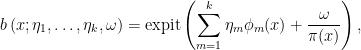
We tentatively model 
with either a smooth or noninformative prior on the parameters 


Of course, this estimator is a clear case of frequentist pursuit Bayes.
7. Conclusion
Here are the main points:
- If
then the posterior will not concentrate.
Thus, if a Bayesian wants the posterior for
he must justify having a prior -
Therefore, an argument of the form: “we want selection bias so we cannot have prior independence” fails. - One can try to argue that prior independence is unrealistic. But as we have shown, this is not the case.
-
But, if after all this, we do insist on letting
it is still not enough. Dependence on
We conclude Bayes fails in our example unless one uses a special prior designed just to mimic the frequentist estimator.
8. Addendum: What happens If The Estimator Does Note Depend on
The theorem of Robins and Ritov, quoted in our initial post, says that no uniformly consistent estimator that does not depend on 


to 

concreteness. In fact, even when we assume
and
improvement in performance.
Given 

and
converges at rate 


explicit estimator. More generally, if 


is constructed in Robins et al (2008) ; Robins et al (2009) prove that the rate cannot be improved on. Given these asymptotic mathematical results, we
doubt any reader can exhibit an estimator, not depending on 
model 
and a sample size of 5,000. By reasonable finite sample performance, we mean an interval estimator that will cover the true
centered on the 
await any candidate estimators, accompanied by at least some simulation
evidence backing up your claim.

9. References
- Robins JM, Tchetgen E, Li L, van der Vaart A. (2009).
Semiparametric Minimax Rates. Electron. J. Statist. Volume 3 (2009),
1305-1321. - Robins JM, Li L, Tchetgen E, van der Vaart A. (2008). Higher order influence
functions and minimax estimation of nonlinear functionals. Probability and
Statistics: Essays in Honor of David A. Freedman 2:335-421 - Robins JM, Ritov Y. (1997). Toward a curse of dimensionality appropriate
(CODA) asymptotic theory for semi-parametric models. Statistics in Medicine,
16:285-319.

13 Comments
I’m disappointed that you didn’t address the questions I asked in response to the previous post. I tracked down the abstract of the Robins-Ritov paper, but the paper itself is behind a paywall. The abstract does not mention the concentration result – could you state it? Does it refer to the rate of convergence of the point estimate to the true value? For the Bayesian inference, which point estimate are you referring to? When you say “the posterior will fail to concentrate”, are you referring to the posterior itself or a point estimate (the posterior mean?) derived from the posterior?
In underspecified problems such as this one, it is generally better to estimate intervals rather than work with point estimates – due to the vast underspecification, a point estimate is almost guaranteed to be far from the true value, but an interval estimate may nonetheless be informative and useful in practice; for instance, hypothesis testing (which essentially relies on interval rather than point estimation) is possible and useful even in overparameterized problems where point estimates are unreliable. Does the concentration result extend in some way to interval estimation?
The Robins-Ritov abstract (like the original post here) refers to properties that estimators must have in order to be _uniformly_ consistent, so I’ll repeat my earlier question: why do you restrict your attention to estimators with this property? Might a pointwise consistent estimator not have better convergence rate?
Yes, in the original post we showed how to get a confidence interval that shrinks . Again, this is possible because of uniform consistency.
at rate
—LW
I do intend to reply. It took us several days to compose our reply to Chris.
Robins and Ritov can be found here
Click to access coda.pdf
–LW
Reply to Konrad
Most of your questions are answered in the references, especially the
Robins-Ritov paper. It would be difficult to discuss all the
technical details in a blog post so I urge you to read the original
papers.
The main points are these: the Robins-Ritov paper proves that any
estimator that is not a function of pi will not concentrate around the
true value. (More precisely, it can only concentrate extremely
slowly). This includes the Bayes estimator since the pi(X_i) terms
drop out of the likelihood (they are know constants).
On the other hand, the Horwitz-Thompson estimator (and its improved
version) are proved to concentrate uniformly at a 1/sqrt{n} rate.
> You point out that the likelihood function contains very little
> information – this is as it should be and provides a sanity check for
> likelihood-based approaches – since there is almost no information
> available about theta, any approach that claims to have access to such
> information should be distrusted.
But the likelihood isn’t the only source of information. The
likelihood ignores the randomization probabilities which are in fact
very informative.
> That said, your argument for the non-informativeness of the
> likelihood function is based on the absence of smoothness
> constraints. You then claim that introducing smoothness
> constraints when the problem is high dimensional will not help
> unless you make the function “very, very, very smooth”- but you
> do not quantify this. The thing to be quantified is not how much
> we know about theta (which remains very little), but how much we
> know about psi (after theta has been marginalised out). On what
> do you base the claim that “we have seen that response 3 doesn’t
> work” when you have made no attempt to quantify how well it
> actually does work or how it compares to your proposed solution?
This is addressed in the addendum (Section 8) to our most recent post.
The amount of smoothness you nee to assume grows quickly with dimension.
> Re priors: given the structure of the problem, and if interesting
> prior information about theta were available to be incorporated into
> the model, it is very feasible that such information would be highly
> dependent on pi – if we imagine this is an experimental setup which
> has been run before and from which we have drawn previous qualitative
> conclusions, those conclusions will have been much more informative
> when pi(x) was mostly large than when it was mostly small, and it
> would make sense to use a prior that is correspondingly tighter for
> larger pi.
Dependence of the prior on pi is necessary but not sufficient to have
the Bayes estimator concentrate around the true value. The prior
needs to be very carefully engineered to get concentration.
> But I agree that one wants results that make sense even when the
> prior is independent of pi (from an objective Bayesian point of
> view, the prior is just another part of the model specification,
> which ought to be specified by the person posing the problem;
> also when we really know nothing about the system there doesn’t
> seem to be any reason to use a prior that depends on pi).
Agreed.
> Finally, it is not clear how desirable uniform consistency (or
> any one specific frequentist metric) is, if (for instance) it is
> obtained at the expense of efficiency. Is a uniformly consistent
> estimator necessarily better than a pointwise consistent
> estimator? (In my limited understanding the main advantage of
> having uniform consistency is that it allows one to establish
> worst case guarantees on confidence interval size for finite
> sample sizes – this is not irrelevant, but one might be more
> interested in optimizing expected rather than worst case error.)
We view uniform consistency as vital. With pointwise consistency, we
can only say that there is some sample size n at which the estimator
becomes accurate to within, say, epsilon. But this n depends on the
unknown theta. With uniform consisency, n depends only on epsilon.
More importantly, without uniform consistency, it’s not possible to
construct a finite sample confidence interval.
I hope these comments help.
—LW
Reply to Enstophy:
You’re right to point out that Bayesians will see probabilities and
frequencies as diferent (although linked via deFinetti’s theorem).
Nonetheless, we consider it reasonable to ask about the frequency
behavior of posteriors probability distributions. Perhaps it would
clearer if we said: one’s posterior beliefs will fail to concentrate
around the truth, in the frequency sense.
I didn’t find your argument that W(theta) should be a function of pi to
be convincing. But anyway, dependence on pi is not enough.
It is necessary but not sufficient.
—LW
There’s a justification for priors carefully engineered to yield uniformly consistent posterior distributions that does not depend on frequentist pursuit per se: it is Solomonoff-induction pursuit. Solomonoff induction does not contradict Bayes and the Solomonoff posterior predictive distribution converges to the sampling distribution with sampling probability one; furthermore, this convergence is at the fastest possible rate. Alas, it is also uncomputable.
If one takes the view that one’s prior ought to be a computable approximation to the Solomonoff prior, these kinds of Freedmanesque inconsistency arguments against Bayes don’t actually militate against Bayes. They are in fact incredibly useful — they show that vast swaths of the space of prior probability distributions can be disregarded, since they do not contain computable approximations to the Solomonoff prior.
This sounds very interesting.
 consistent.
I would like to see a prof that in this example
it yields an estimator that is uniformly
—LW
I’ve posted a round 4 now. I show that the simple example in the last post by Robins and Wasserman does not make the point that it claims to make. The arguments they want to make do depend fundamentally on infinite dimensionality, I think, and I should try to look at the Robins-Ritov reference and respond directly to that. But, for a while, maybe days, I have other stuff to get done. All my posts are still at http://sims.princeton.edu/yftp/WassermanExmpl.
For the problem to arise, it seems theta(x.i) must be not smooth enough for theta(x.i) ~ theta(x.j) i != j for any (or at least most) i , j where R = 1 (where Y is observed), the interest must be in psy, the E[Y] a _uniform_ expectation over [0,1]^d and pi(x) must be both non-informative (given x) and non-uniform from [0,1]^d when R=1. There does not seem to be a problem about the posterior of theta(x.i) which is simply a mixture of the prior of theta(x.i|x.i.obs,R=1,Y) or prior of theta(x.i|x.i.obs,R=0 )~ prior of theta(x.i|x.i.obs) (i.e. a mixture of posterior and prior with most of it being prior). The problem arises integrating this posterior over [0,1]^d for psy as the target and it is not clear in the blog post how this is done. Simply collapsing the posterior over x.i.obs[just where R=1] (non uniform) would seem very wrong
.
This would explain why pi(x)=1/2 for all x does not cause any problem to arise, x.i.obs will be uniform and why a prior with all the mass on a linear function for theta(x.i) (or any combination of polynomials that is linear in x.i) will not cause a problem – the parameter(s) are the same (e.g. alpha) anywhere in [0,1]^d and a non-uniform sample from [0,1]^d does not create problem if large enough (non-singular).
As for the comment “If you want to be a Bayesian, be a Bayesian but accept the fact that, in this example, your posterior will fail to concentrate around the true value.” given the study design analogy of purposely choosing to sample with pi(x.i), for the objective of estimating psi, given non-smooth theta(x.i), the design is flawed for the usual Bayesian analysis and it perhaps should not be surprising that a fix is not easy to come up with. HT is designed to fix just this problem, and the Bayesian should perhaps not feel bad pronouncing that they can do nothing Bayesian for the patient except to pronounce them dead.
So this goes in my bin of stuff that is ignorable for the practicing statistician (unlike Neyman-Scott).
Or I may still not unstand their example well enough….
Hi there,
in 2007, Marc Toussaint and I wrote a Technical Report about “Bayesian
estimators for Robins-Ritov’s problem” [http://eprints.pascal-network.org/archive/00003871/01/harmeling-toussaint-07-ritov.pdf] which includes simulations
and which also concludes that the critical point is the dependence
or independence of theta and pi. In Section 3 and 4, we considered the
setting X.i ~ uniform(1…C), R.i ~ bernoulli(pi.i), Y.i ~ N(R.i *
theta.i, 1).
(i) In Section 3 we derive a Bayesian estimator that does not assume
dependence between theta and pi (in our report xi). A simulation
shows that this Bayesian estimator has a smaller variance than the
Horwitz-Thompson (HT) estimator on data that has been generated with
independent theta and pi. Thus for such data the Bayesian estimator
has no problems (even has lower variance).
(ii) In Section 4 we assume that theta and pi are dependent. To
derive a Bayesian estimator we have to model this dependence. Of
course there are many possibilities: we choose a dependency that
relates to the dependency used in Robins and Ritov (1997) in their
proof that a likelihood-based estimator can not be uniformly unbiased.
The Bayesian estimator looks quite similar to the HT estimator.
However, on simulated data that follows this model the Bayesian
estimator has again a lower variance. So also for the dependent case,
the Bayesian estimator derived from the model assumptions (dependence
of theta and pi) works. Curiously, it also weights the samples
similar to the HT estimator.
(iii) Section 5 shows that similar arguments hold for continuous X.
My conclusion has three points (which might be obvious by now):
(1) The HT estimator works only good on data where theta and pi are
dependent. The advantage of the HT estimator might be that this
dependence does not have to be made explicit.
(2) If the dependence between theta and pi can be made explicit, we
can derive a Bayesian estimator which works as well as the HT
estimator (possibly with lower variance). The disadvantage of the
Bayesian approach might be that the dependence has to be made
explicit.
(3) The third point is a question: can we exploit a possible
dependence between theta and pi in a Bayesian estimator without making
it explicit?
I’d be curious to hear the experts’ opinion on these thoughts! Thanks!
will take a look and get back to you
LW
Interesting, though you might be interesting in looking at Neyman-Scott discussion in Barndorff-Nielsen, O., and Cox, D. R. Inference and asymptotics. Chapman and
Hall, London, 1994.
Where they argue that, essentially the approaches to salvage the likelihood
separate into two, one is to … and the second replaces the specification of arbitrary
non-commonness of the non-common parameter with a common distribution for that parameter [i.e. latent generative model].
Still unclear to me, what compels one to take certain summaries of the posterior over others…
I’ve posted a (final?) comment on this at the same place as the earlier one (sims.princeton.edu/yftp/WassermanExmpl). It’s the WassermanR4a.pdf file. It repeats some of what I’ve said earlier, but tries to build up the discussion from simple examples to the continuous case.