The Remarkable k-means++

1. The Problem

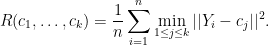
One of the most popular algorithms for clustering is k-means. We start with ${n}$ data vectors ${Y_1,\ldots, Y_n\in \mathbb{R}^d}$ . We choose ${k}$ vectors — cluster centers — ${c_1,\ldots, c_k \in \mathbb{R}^d}$ to minimize the error

$\displaystyle R(c_1,\ldots,c_k) = \frac{1}{n}\sum_{i=1}^n \min_{1\leq j \leq k} ||Y_i - c_j||^2.$

Unfortunately, finding ${c_1,\ldots, c_k}$ to minimize ${R(c_1,\ldots,c_k)}$ is NP-hard. The usual iterative method, \hrefnosnap{http://en.wikipedia.org/wiki/Lloyd is easy to implement but it is unlikely to come close to minimizing the objective function. So finding

$\displaystyle \min_{c_1,\ldots, c_k}R(c_1,\ldots,c_k)$

isn’t feasible.

To deal with this, many people choose random starting values, run the ${k}$ -means clustering algorithm then rinse, lather and repeat. In general, this may work poorly and there is no theoretical guarantee of getting close to the minimum. Finding a practical method for approximately minimizing ${R}$ is thus an important practical problem.

2. The Solution

David Arthur and Sergei Vassilvitskii came up with a wonderful solution in 2007 known as k-means++.

The algorithm is simple and comes with a precise theoretical guarantee.

The first step is to choose a data point at random. Call this point ${s_1}$ . Next, compute the squared distances

$\displaystyle D_i^2 = ||Y_i - s_1||^2.$

Now choose a second point ${s_2}$ from the data. The probability of choosing ${Y_i}$ is ${D_i^2/\sum_j D_j^2}$ . Now recompute the distance as

$\displaystyle D_i^2 = \min\Bigl\{ ||Y_i - s_1||^2, ||Y_i - s_2||^2 \Bigr\}.$

Now choose a third point ${s_3}$ from the data where the probability of choosing ${Y_i}$ is ${D_i^2/\sum_j D_j^2}$ . We continue until we have ${k}$ points ${s_1,\ldots,s_k}$ . Finally, we run ${k}$ -means clustering using ${s_1,\ldots,s_k}$ as starting values. Call the resulting centers ${\hat c_1,\ldots, \hat c_k}$ .

Arthur and Vassilvitskii prove that

$\displaystyle \mathbb{E}[R(\hat c_1,\ldots,\hat c_k)] \leq 8 (\log k +2) \min_{c_1,\ldots, c_k}R(c_1,\ldots,c_k).$

The expected value is over the randomness in the algorithm.

There are various improvements to the algorithm, both in terms of computation and in terms of getting a sharper performance bound.

This is quite remarkable. One simple fix, and an intractable problem has become tractable. And the method comes armed with a theorem.

3. Questions

Is there an R implementation? It is easy enough to code the algorithm but it really should be part of the basic k-means function in R.
Is there a version for mixture models? If not, it seems like a paper waiting to be written.
Are there other intractable statistical problems that can be solved using simple randomized algorithms with provable guarantees? (MCMC doesn’t count because there is no finite sample guarantee.)

4. Reference

Arthur, D. and Vassilvitskii, S. (2007). k-means++: The advantages of careful seeding. Proceedings of the eighteenth annual ACM-SIAM symposium on Discrete algorithms. 1027–1035.

This entry was written by normaldeviate, posted on September 30, 2012 at 8:19 pm, filed under Uncategorized. Bookmark the permalink. Follow any comments here with the RSS feed for this post. Both comments and trackbacks are currently closed.

10 Comments

John Myles White

Posted September 30, 2012 at 9:46 pm | Permalink

Great post. Looks like \hrefnosnap{http://en.wikipedia.org/wiki/K-means might need to be changed to \hrefnosnap{http://en.wikipedia.org/wiki/K-means} or something similar.
Ar

Posted October 1, 2012 at 6:20 am | Permalink

Does it always find an optimal solution ?
normaldeviate

Posted October 1, 2012 at 8:25 am | Permalink

Fixed. Thanks.
Christian Hennig

Posted October 1, 2012 at 12:47 pm | Permalink

The idea is nice and the result is brilliant. Still, a theoretical guarantee is not a practical one. Did they confirm by simulations that this is really better than “many random starts” or some of the other heuristical stuff that has been proposed for this?

Regarding mixture models, the problem in the Gaussian case is that if you have models where you allow for different covariance matrices within clusters, the whole thing cannot be goverened anymore by a single distance measure, because for different clusters different Mahalanobis distances would be required. So it would be less straightforward. Roughly related problems would occur with mixtures of skew distributions, also to do with the fact that “effective distance” is not the same everywhere in data space, as it is for k-means.
- normaldeviate
  
  Posted October 1, 2012 at 1:48 pm | Permalink
  
  My own (limited) experience is that it works very well.
Geoff Gordon

Posted October 1, 2012 at 12:53 pm | Permalink

A nice related result:

http://arxiv.org/abs/1206.5766

Hsu and Kakade show a consistent estimator for mixtures of spherical Gaussians, based on a spectral algorithm. So, if we want to run k-means because we’re trying to estimate this particular model, then in the limit, we actually can get much better performance than the guarantee above. (Of course, k-means doesn’t estimate exactly this model, and there are other reasons to run k-means besides trying to estimate this model.)
- zkolter
  
  Posted October 2, 2012 at 9:01 am | Permalink
  
  One notable criterion for the Hsu and Kakade algorithm is that the dimensionality of the data much be larger than the number of clusters, d > k. I recall you had mentioned it might be possible to remove this restriction from the HMM case (by concatenating observations? I wasn’t quite clear how this would work…), but it seems fairly central to the mixture of Gaussians case. A great algorithm for the cases when it applies, but a nice feature of k-means++ is that it isn’t dependent on the input dimension.
  
  Practically speaking, the nice thing about km++ is that it’s extremely simple to implement and in my experience does work significantly better than many random initializations. It doesn’t necessarily work that much better than the wealth of other possible ways of initializing cluster centroids (basically all takes on low-dispersion sampling, which is also what km++ is doing), but the fact that is has a very elegant theory and is easy to implement makes me typically use it for initializing k-means.
  - normaldeviate
    
    Posted October 2, 2012 at 9:07 am | Permalink
    
    Take nine spherical Gaussians in the plane with ceneters place like this:
    
    X X X
    
    X X X
    
    X X X
    
    You get nine nice clusters. k-means with random starts has essentially 0 probability of getting the right clusters
    but k-meas++ seems to nail it!
    –LW
  - Geoff Gordon
    
    Posted October 6, 2012 at 2:17 pm | Permalink
    
    Yes, the d >= k restriction is a pain. It is possible to remove it for the HMM case, by taking features of histories longer than 1 observation. (E.g., for an HMM with transition matrix T and observation matrix O, if we start in belief state x, the observation probabilities for the next few steps are Ox, OTx, OTTx, etc. If O has fewer rows than columns, then the observation probabilities at a single time step don’t determine x, but taking probabilities for several successive steps will determine x.)
    
    However, I don’t see how to use this trick for Gaussian mixtures, since we only ever get one view of a particular latent variable (in contrast to HMMs, where all future observations are potentially influenced by the current state).
    
    It is possible to make a good density estimate in the case of more centers than dimensions (e.g., by estimating the kernel mean map), but this method doesn’t satisfy one of the main use cases of k-means, which is that someone actually wants to know the center locations.
Luis Leiva

Posted October 12, 2012 at 6:00 am | Permalink

See ‘Pattern Classification. R.O. Duda, P.E. Hart & D.G. Stork’.

2 Trackbacks

By Economist's View: Links for 10-01-2012 on October 1, 2012 at 3:08 am

[…] The Remarkable k-means++ (Quadruple wonk alert) – Normal Deviate […]
By The Value of Adding Randomness « Normal Deviate on June 9, 2013 at 10:23 am

[…] Minimizing the objective function in -means clustering is NP-hard. Remarkably, as I discussed here, the -means++ algorithm uses a careful randomization method for choosing starting values and gets […]

Normal Deviate