Bootstrapping and Subsampling: Part I

BOOTSTRAPPING AND SUBSAMPLING: PART I

Bootstrapping and subsampling are in the “amazing” category in statistics. They seem much more popular in statistics than machine learning for some reason.

1. The Bootstrap

The bootstrap (a.k.a. the shotgun) was invented by Brad Efron. Here is how it works. We have data ${X_1,\ldots, X_n \sim P}$ and we want a confidence interval for ${\theta = T(P)}$ . For example, ${\theta}$ could be the median of ${P}$ or the mean of ${P}$ or something more complicated like, the largest eigenvalue of the covariance matrix of ${P}$ .

The ${1-\alpha}$ bootstrap confidence interval is

$\displaystyle C_n = \left[ \hat\theta - \frac{\hat t_{1-\alpha/2}}{\sqrt{n}},\ \hat\theta - \frac{\hat t_{\alpha/2}}{\sqrt{n}}\right]$

where ${\hat\theta}$ is an estimator of ${\theta}$ and ${\hat t_{\alpha/2}}$ and ${\hat t_{1-\alpha/2}}$ are sample bootstrap quantiles that I will describe below. Before I explain this in more detail, notice two things. First, there is a minus sign in both the lower and upper endpoint. Second, the ${\alpha/2}$ and ${1-\alpha/2}$ quantiles are in the upper and lower endpoints, the reverse of what you might expect. The reason for the strange looking interval will be clear when we derive the interval.

Now for some details. Think of the parameter of interest ${\theta}$ as a function of the unknown distribution, which is why we write it as ${\theta = T(P)}$ . Let ${P_n}$ denote the empirical distribution:

$\displaystyle P_n(A) = \frac{1}{n}\sum_{i=1}^n I_A(X_i).$

In other words, ${P_n}$ is the distribution that puts mass ${1/n}$ at each ${X_i}$ .

The estimator is just the function ${T}$ applied to ${P_n}$ , that is, ${\hat\theta = T(P_n)}$ . For example, if ${\theta}$ is the median of ${P}$ then ${\hat\theta}$ is the median of ${P_n}$ which is just the sample median.

Now let

$\displaystyle R_n = \sqrt{n}(\hat\theta - \theta).$

We use ${R_n}$ because typically it converges in distribution to some well-defined distribution (such as a Normal). Now let ${H_n}$ denote the (unknown) distribution of ${R_n}$ :

$\displaystyle H_n(t) = \mathbb{P}(R_n \leq t).$

Suppose, for a moment, that we did know ${H_n}$ . We could then find the ${\alpha/2}$ quantile ${t_{\alpha/2}}$ and the ${1-\alpha/2}$ quantile ${t_{1-\alpha/2}}$ , namely,

$\displaystyle t_{\alpha/2} = H_n^{-1}(\alpha/2)\ \ \ \mbox{and}\ \ \ t_{1-\alpha/2} = H_n^{-1}(1-\alpha/2).$

It follows that

$\displaystyle \mathbb{P}( t_{\alpha/2} \leq R_n \leq t_{1-\alpha/2}) = 1- \alpha.$

Continuing with the fantasy that we know ${H_n}$ , define

$\displaystyle \Omega_n = \left[ \hat\theta - \frac{t_{1-\alpha/2}}{\sqrt{n}},\ \hat\theta - \frac{t_{\alpha/2}}{\sqrt{n}}\right].$

Now I will show you that ${\Omega_n}$ is an exact ${1-\alpha}$ confidence interval. This follows since

$\displaystyle \mathbb{P}(\theta \in \Omega_n) = \mathbb{P}\left(\hat\theta - \frac{t_{1-\alpha/2}}{\sqrt{n}} \leq \theta \leq \hat\theta - \frac{t_{\alpha/2}}{\sqrt{n}}\right)= \mathbb{P}(t_{\alpha/2} \leq R_n \leq t_{1-\alpha/2}) = H_n(t_{1-\alpha/2}) - H_n(t_{\alpha/2})= (1-\alpha/2) - \alpha/2 = 1-\alpha.$

We engineered ${\Omega_n}$ so that the last line would be exactly ${1-\alpha}$ . The strange form of ${\Omega_n}$ is explained by the fact that we really have a probability statement for ${R_n}$ which we then manipulate into the form of an interval for ${\theta}$ . (You can check that if ${H_n}$ were standard Gaussian, then using the symmetry of the Gaussian, the interval could be re-written in the more familiar looking form ${\hat\theta\pm z_{\alpha/2}/\sqrt{n}}$ where ${z_{\alpha/2}}$ is the upper-tail quantile of a Normal.)

The problem is that we don’t know ${H_n}$ and hence we don’t know ${t_{\alpha/2}}$ or ${t_{1-\alpha/2}}$ . The bootstrap is a method for approximating ${H_n}$ . Let ${B}$ be a large number (for example, ${B=100,000}$ .) Now do this:

Draw ${n}$ observations ${X_1^*,\ldots, X_n^*}$ from ${P_n}$ and compute ${\hat\theta^*}$ from these new data.
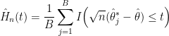
Repeat step 1 ${B}$ times yielding values ${\hat\theta_1^*,\ldots, \hat\theta_B^*}$ .
Approximate ${H_n}$ with
$\displaystyle \hat H_n(t) = \frac{1}{B}\sum_{j=1}^B I\Bigl( \sqrt{n}(\hat\theta_j^* - \hat\theta)\leq t\Bigr)$

where ${I}$ denotes the indicator function.
Find the quantiles ${\hat t_{\alpha/2}}$ and ${\hat t_{1-\alpha/2}}$ of ${\hat H_n}$ and construct ${C_n}$ as defined earlier.

The interval ${C_n}$ is the same as ${\Omega_n}$ except we use the estimated quantiles for ${C_n}$ . What we are doing here is estimating ${H_n}$ by using ${P_n}$ as an estimate of ${P}$ . (That’s why we draw ${X_1^*,\ldots, X_n^*}$ from ${P_n}$ .) If ${\hat H_n}$ is close to ${H_n}$ then ${\hat t_{\alpha/2} \approx t_{\alpha/2}}$ and ${\hat t_{1-\alpha/2} \approx t_{1-\alpha/2}}$ and then ${C_n \approx \Omega_n}$ .

There are two sources of error. First we approximate

$\displaystyle H_n(t)=\mathbb{P}(\sqrt{n} (\hat\theta - \theta))$

with

$\displaystyle H_n^*(t)=\mathbb{P}_n(\sqrt{n} (\hat\theta^* - \hat\theta)).$

Essentially, we are replacing ${P}$ with ${P_n}$ . Second, we are approximating ${H_n^*(t)}$ with

$\displaystyle \hat H_n(t) = \frac{1}{B}\sum_{j=1}^B I\Bigl( \sqrt{n}(\hat\theta_j^* - \hat\theta)\leq t\Bigr).$

This second source of error is negligible because we can make ${B}$ as large as we want.

Remark: A moment’s reflection should convince you that drawing a sample of size ${n}$ from ${P_n}$ is the same as drawing ${n}$ points with replacement from the original data. This is how the bootstrap is often described but I think it is clearer to describe it as drawing ${n}$ observations from ${P_n}$ .

2. Why Does It Work?

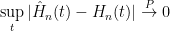
If ${\hat H_n}$ is close to ${H_n}$ then the bootstrap confidence interval will have coverage close to ${1-\alpha}$ . Formally, one has to show that

$\displaystyle \sup_t |\hat H_n(t) - H_n(t)| \stackrel{P}{\rightarrow} 0$

in which case

$\displaystyle \mathbb{P}(\theta\in C_n) \rightarrow 1-\alpha$

as ${n\rightarrow\infty}$ .

It is non-trivial to show that ${\sup_t |\hat H_n(t) - H_n(t)| \stackrel{P}{\rightarrow} 0}$ but it has been shown in some generality. See Chapter 23 of van der Vaart (1998) for example.

3. Why Does It Fail?

The bootstrap does not always work. It can fail for a variety of reasons such as when the dimension is high or when ${T}$ is poorly behaved.

An example of a bootstrap failure is in the problem of estimating phylogenetic trees. The problem here is that ${T(P)}$ is an extremely complex object and the regularity conditions needed to make the bootstrap work are unlikely to hold.

In fact, this is a general problem with the bootstrap: it is most useful in complex situations, but these are often the situations where the theory breaks down.

4. What Do We Do?

So what do we do when the bootstrap fails? One answer is: subsampling. This is a variant of the bootstrap that works under much weaker conditions than the bootstrap. Interestingly, the theory behind subsampling is much simpler than the theory behind the bootstrap. The former involves little more than a simple concentration inequality while the latter uses high-powered techniques from empirical process theory.

So what is subsampling?

Stay tuned. I will describe it in my next post. In the meantime, I’d be interested to hear about your experiences with the bootstrap. Also, why do you think the bootstrap is not more popular in machine learning?

References

Efron, Bradley. (1979). Bootstrap methods: Another look at the jackknife. The Annals of Statistics, 1-26.

Efron, Bradley, and Tibshirani, R. (1994). An Introduction to the Bootstrap. Chapman and Hall.

Holmes, Susan. (2003). Bootstrapping phylogenetic trees: Theory and methods. Statistical Science, 241-255.

van der Vaart, A. (1996). Asymptotic Statistics. Cambridge.

P.S. See also Cosma’s post:
here

10 Comments

Alex

Posted January 20, 2013 at 12:27 pm | Permalink

I think machine learning people do not care about confidence interval too much in general.
Vainius

Posted January 21, 2013 at 3:35 am | Permalink

In the bootstrap confidence interval do we put estimate of theta from original data, or do we put mean of all bootstrap estimates there? Generally they should be the same, but there are cases where they can differ (e.g. when T is median).
- normaldeviate
  
  Posted January 29, 2013 at 11:02 am | Permalink
  
  the original
Geoff Gordon

Posted January 21, 2013 at 10:32 am | Permalink

I think one reason the bootstrap isn’t more popular is what Larry mentioned: “it is most useful in complex situations, but these are often the situations where the theory breaks down”. (There’s not much point in going to a lot of effort to get an error bound if the error bound is probably wrong.) Another is that the bootstrap requires re-running your estimation procedure a very large number of times, and often in ML we’re lucky if we can run the estimation procedure once.
Christian Hennig

Posted January 21, 2013 at 10:35 am | Permalink

I like bootstrap and use it occasionally. However, I think that an important issue with (nonparametric) bootstrap is that some features of P_n are essentially different from P (or our typical idea of P). P_n is basically discrete. This has implications. For example, in clustering, samples from P_n tend to produce larger between-cluster separation than the original sample, because points that could spoil separation can be taken away, but never added. Producing multiple points at the same location can lead to artifacts in clustering, but also in covariance-matrix estimation or group-wise covariance matrices in classification (implosion of eigenvalues). Samples from P_n (with or without multiple points) can have a smaller but not larger convex hull then the original samples etc. So I’d say that one needs to be very careful with bootstrapping statistics that can somehow be affected by discreteness, the convex hull and other problematic features somebody else comes up with.
- rj444
  
  Posted January 21, 2013 at 2:28 pm | Permalink
  
  Yes, I was confused by the comment – “A moment’s reflection should convince you that drawing a sample of size n from Pn is the same as drawing n points with replacement from the original data”. The adequacy of the Pn approximation is exactly what I have trouble convincing myself of even after a moment’s reflection, especially when n is relatively small and T(P) is relatively complex.
  
  I find it interesting that Larry says “an example of a bootstrap failure is in the problem of estimating phylogenetic trees”. In practice this is one of the areas where boostrap is used most often.
  - normaldeviate
    
    Posted January 21, 2013 at 2:32 pm | Permalink
    
    P_n is a very accurate estimate of P
    This follows from standard empirical process theory
    For example, in one-dimension, P( ||P_n – P||_infty > epsilon) < 2e^{-2n epsilon^2}
    
    The issue is the behavior of T(P).
  - Christian Hennig
    
    Posted January 21, 2013 at 6:11 pm | Permalink
    
    n is not always large, though.
  - Martin Azizyan
    
    Posted January 23, 2013 at 5:46 am | Permalink
    
    rj444, I believe the “original data” in the statement “drawing a sample of size n from Pn is the same as drawing n points with replacement from the original data” refers to the finite sample we were given, not the true distribution. This is not a statistical claim. It follows from the definitions of the empirical distribution and of sampling with replacement.
    
    I think that’s what you were asking, but I’m sorry if I misunderstood the subject of your confusion.
Keith O'Rourke

Posted January 21, 2013 at 1:12 pm | Permalink

I prefer to think of the bootstrap as sampling paths from the product space Pn(A)^n WITH replacement which is less efficient than without replacement, but that very quickly decreases with increasing “n”.

Makes it teachable as simple survey sampling, which worked well with undergrad class once. But the BCA correction stuff and why it fails for complex problems seemed way too hard to get accross.

Remember Efron wrote a paper in the early 2000 complaining most statisticians actual do bootstrapping incorrectly.

That included me, in that when the percentile intervals were _simmilar_ to the BCA intervals in applications, I (mis)thought they had no advantage (i.e. I forgot to think about the distribution of intervals over repeated applications).

5 Trackbacks

By Bootstrap e Subamostragem | Mineração de Dados on January 20, 2013 at 8:50 am

[…] um ótimo post do Normal Deviate sobre o […]
By Weekly Digest – January 20, 2013 | Robust Analysis on January 20, 2013 at 10:02 pm

[…] Larry Wasserman, Bootstrapping and Subsampling, Part I: […]
By Bootstrapping and Subsampling: Part II « Normal Deviate on January 27, 2013 at 9:02 am

[…] « Bootstrapping and Subsampling: Part I […]
By Comunidades tribais são mais violentas? O quão próxima é a distribuição normal? O papel do BNDES. | Análise Real on February 4, 2013 at 8:14 pm

[…] Sobre bootstraping I e […]
By The Value of Adding Randomness « Normal Deviate on June 9, 2013 at 10:23 am

[…] The Bootstrap. I discussed the bootstrap here. Basically, to compute a confidence interval, we approximate the […]

Normal Deviate