Super-efficiency: The Nasty, Ugly Little Fact
I just read Steve Stigler’s wonderful article entitled: “The Epic Story of Maximum Likelihood.” I don’t know why I didn’t read this paper earlier. Like all of Steve’s papers, it is at once entertaining and scholarly. I highly recommend it to everyone.
As the title suggests, the paper discusses the history of maximum likelihood with a focus on Fisher’s “proof” that the maximum likelihood estimator is optimal. The “nasty, ugly little fact” is the problem of super-efficiency.
1. Hodges Example
Suppose that
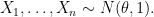
The maximum likelihood estimator (mle) is

We’d like to be able to say that the mle is, in some sense, optimal.
The usual way we teach this, is to point out that 
Hodges’ famous example shows that this is not quite right. Hodges’ estimator is:
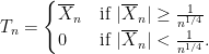
If 


But if 

![{[-n^{-1/4},n^{-1/4}]}](https://s0.wp.com/latex.php?latex=%7B%5B-n%5E%7B-1%2F4%7D%2Cn%5E%7B-1%2F4%7D%5D%7D&bg=ffffff&fg=000000&s=0&c=20201002)


Hence, the mle is not optimal, at least, not in the sense Fisher claimed.
2. Rescuing the mle
Does this mean that the claim that the mle is optimal is doomed? Not quite. Here is a picture (from Wikipedia) of the risk of the Hodges estimator for various values of 

There is a price to pay for the small risk at
First, if we look at the maximum risk rather than the pointwise risk then we see that the mle is optimal. Indeed,
Second, Le Cam showed that the mle is optimal among all regular estimators. These are estimators whose distribution is not affected by small changes in the parameter. This is known as Le Cam’s convolution theorem because he showed that the limiting distribution of any regular estimator is equal to the distribution of the mle plus (convolved with) another distribution. (There are, of course, regularity assumptions involved.)
Chapter 8 of van der Vaart (1998) is a good reference for these results.
3. Why Do We Care?
The idea of all of this, was not to rescue the claim that “the mle is optimal” at any cost. Rather, we had a situation where it was intuitively clear that something was true in some sense but it was difficult to make it precise.
Making the sense in which the mle is optimal precise represents an intellectual breakthrough in statistics. The deep mathematical tools that Le Cam developed have been used in many aspects of statistical theory. Two reviews of Le Cam theory can be found here and here.
That the mle is optimal seemed intuitively clear and yet turned out to be a subtle and deep fact. Are there other examples of this in Statistics and Machine Learning?
References
Stigler, S. (2007). The epic story of maximum likelihood. Statistical Science, 22, 598-620.
van der Vaart. (1998). Asymptotic Statistics. Cambridge.
van der Vaart, Aad. (2002). The statistical work of Lucien Le Cam. Ann. Statist., 30, 631-682.

17 Comments
Not to diminish LeCam’s contributions to this area because they were absolutely fundamental, but I believe the Convolution Theorem is due to Jaroslav Hajek.
You are correct of course Keith, thanks.
I should have called it the Hajek-LeCam theorem.
By the way, here is the wikipedia link for the theorem:
http://en.wikipedia.org/wiki/H%C3%A1jek%E2%80%93Le_Cam_convolution_theorem
I have been working on estimation for the Generalized Laplace distribution (or Variance gamma https://en.wikipedia.org/wiki/Variance-gamma_distribution).
If \lambda < 0.5 (using the notation from the wikipedia link) the likelihood of a set of observations X_1, X_2, \ldots ,X_n is unbounded for \mu (the location parameter) at the points X_1,X_2,\ldots,X_n. So the mle is unmodfied wont work for the distribution.
Yes there are many examples where maximum likelihood fails.
The problem is to identify what it means precisely to say
what “optimal” means and under what conditions is the mle optimal.
Finding the Maximum Likelihood Estimator is equivalent (in distributions from the Exponential Family) to maximizing the entropy subject some constraint and then using the method of the Lagrange Multipliers to handle the constraints. One might object that this only applies to distributions from the Exponential Family, but sense that includes all the common distributions wherein MLE is usually applied without problems, and it seems to run into trouble outside that range, then it’s enough to make you wonder if entropy isn’t the key. Maybe “Maximizing Entropy” is the relevant optimality requirement for MLE’s.
No. I think LeCam theory
is the relevant optimality.
He nailed it.
Well sinse they’re both thoerems I guess it’s a matter of taste who nailed it. The maximum entropy approach makes sense because what’s really going on is that by maximizing the entropy, you’re maximizing the size of high probability manifold of the distribution thereby created the greatest opportunity possible for the true value to be in the high probability manifold. Since that’s what’s really required to make reliable inferences, it’s all kinds of relevant. That’s all very Bayesian though.
There’s no need to be either/or however. Have you considered the possibility that they’re related? How closely connected is the class of distributions with regular estimators to class of Maximun entropy distributions using their sufficient statistics as the estimator? Although they seem completely different, I wouldn’t be surprised if they were connected. The class of maximum entropy distributions and class of distributions with sufficient statistics seemed completely unrelated until they were proven to be identical.
The exponential family is a very special case.
The connections of LeCam theory to exponential families
have been well understood for a very long time.
Why not just study LeCam theory? You might find it interesting.
I will definitely after see this.
Do you mean “bowl-shaped loss functions”? It’s a bit odd to refer to bowl-shaped estimators.
Yes! Thanks
Also a bit surprised not to see Stein estimators mentioned… doing better than the MLE, at least in some sense.
I was saving that for another day
Looking forward to the Stein estimators post
I recall the Neyman-Scott stuff being central in Stephen’s paper – just too well known to be of interest?
yes, an interesting example, indeed
Larry: I had read a previous draft and it turns out that the couple pages on Neyman-Scott being the main defeat of Fisher’s likelihood method has been reduced to a few comments in the published version. Apparently Stephen changed his mind, though as the most important practical problem he still goes with Neyman-Scott.
One Trackback
[…] plotted the risk function of the Hodges estimator here. The risk of the mle is flat. The large peaks in the risk function of the Hodges estimator are very […]