The Tyranny of Tuning Parameters
We all know about the curse of dimensionality. The curse creates serious practical and theoretical difficulties in many aspects of statistics. But there is another pernicious problem that gets less attention. I call it: The Tyranny of Tuning Parameters.
Many (perhaps most) data analysis methods involve one or more tuning parameters. Examples are: the 
For some of these problems we have good data-driven methods to choose the parameters. But for others we don’t. For example, the optimal choice of tuning parameter for the lasso requires knowledge that we would never have in practice.
1. Regression: A Success
An example of a success is cross-validation in regression. Here is one version. Suppose the data are 


If 

Minimizing the prediction error is the same as minimizing the 

where 
Estimate the risk using the test set:
Choose 


Let 


where

and

In words: if you use cross-validation to use the tuning parameter 
(Note: I focused on sample splitting but of course there are lots of other versions of cross-validation: leave-one-out, 10 fold etc.)
This is an example of a successful data-driven method for choosing the tuning parameter. But there are caveats. The result refers only to prediction error. There are other properties we might want; I’ll save that for a future post.
2. Density Estimation: A Failure
Now consider density estimation. Let 


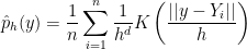
where 

We want to choose

which is equivalent to minimizing

The latter can be estimated using test data 

If we choose 


for a constant 

This is a nice result. Like the regression result above, it gives us assurance that cross-validation (data-splitting) chooses a good tuning parameter.
But, I don’t think cross-validation really does solve the bandwidth selection problem in density estimation. The reason is that I don’t think
Look at these three densities:

In this case, 


Another example is shown in the following plot:

The top left plot is the true distribution which is a mixture of a bimodal density with a point mass at 0. Of course, this distribution is singular; it does not really have a density. The top right shows the density estimator with a small bandwidth, the bottom left shows the density estimator with a medium bandwidth and the bottom right shows the density estimator with a large bandwidth. I would call the estimator in the bottom left plot a success; it shows the structure of the data nicely. Yet, cross-validation leads to the choice 
Despite years of research, I don’t think we have a good way to choose the bandwidth in a sample problem like density estimation.
3. Scale Space
Steve Marron takes a different point of view (Chaudhuri and Marron, 2002). Borrowing ideas from computer vision, he and his co-authors have argued that we should not choose a bandwidth. Instead, we should look at all the estimates 
I have much sympathy for this viewpoint. And it is similar to Christian Hennig’s views on clustering.
Nevertheless, I think in many cases it is useful to have a data-driven default value and I don’t think we have one yet.
4. Conclusion
There are many other examples where we don’t convincing methods for choosing tuning parameters. In many journal and conference papers, the tuning parameters have been chosen in a very ad-hoc way to make the proposed method look successful.
In my humble opinion, we need to put more effort into finding data-driven methods for choosing these annoying tuning parameters.
5. References
Gy\”{o}rfi, Kohler, Krzy\'{z}ak and Walk. (2002). A Distribution-free Theory of Nonparametric Regression.
Chaudhuri, P. and Marron, J.S. (2000). Scale space view of curve estimation. The Annals of Statistics, 28, 408-428.
Wegkamp, M.H. (1999). Quasi-universal bandwidth selection for kernel density estimators. Canadian Journal of Statistics, 27, 409-420.
— Larry Wasserman

12 Comments
> The result refers only to prediction error. There are other properties we might want; I’ll save that for a future post.
This would be interesting. Can there be something that goes beyond empirical prediction?
sure. like support recovery.
I’ll post about that soon
–LW
Very good post! For me, one of the reasons for the recent popularity of shape constrained density estimation, like log-concave densities, is that the choice of a tuning parameter becomes unnecessary!
This area is very promising, at least as I see it.
Also, whenever dealing with testing procedures, the choice of the tuning parameter becomes even more serious since there is no clear way of choosing an appropriate loss function.
I quite like the post! Very good and didactic.
That’s true. Shape constrained density estimation is often tuning parameter free which
is nice.
Nice that you mention my view on cluster analysis; if people want to read about it, something is here (still in “submitted” state):
Click to access mixedsocialcluster1111.pdf
The essence of my view is that I think that scientists want to be “objective”, which far too often tempts them into not deciding things that need to be decided. Not everything can be done data-driven. If you have a loss function, OK, the data can help you to optimise it. But the data can’t tell you which loss function to choose, and so the data really can’t tell you whether you should be interested in squared loss or some other loss, which actually depends on what you want to do with the result. In density estimation, really the scientist needs to decide how much smoothness he or she wants. The data can’t decide this because smoothness of a density is strictly not observable.
In cluster analysis, if you have two nicely separated Gaussian mixture components and move them closer and closer to each other, at some point this will look like a single cluster, not two. And the researcher has to decide from which cutoff downwards this should be treated as a single cluster. There is no way the data can do this (OK, you could test unimodality but in several applications this is not the cluster concept you’re after). So there is no way to have the data properly decide the number of clusters without any kind of tuning. We should actually *want* to tune things so that they are of use to us (this assumes that it is well understood what tuning constants do, so I’m still in favour of getting rid of them where it’s not).
Something about loss function in this spirit is
C. Hennig and M. Kutlukaya: Some thoughts about the design of loss functions. REVSTAT 5 (2007), 19-39 (freely available online).
Thanks for another great thought provoking post. I don’t see why the density estimation failure is an example of the tyranny of tuning parameters, though. It seems to stem purely from the loss function. Are there examples where cross validation is known to not necessarily choose a good tuning parameter asymptotically or in practice given a loss function?
Thanks for a nice post! One interesting question that it brings to mind is how to compare a plain training / validation-set split vs. cross-validation. One would hope that k-fold cross-validation would admit tighter generalization bounds than just using some fraction of the data as a validation set for picking the tuning parameter.
Another interesting question is the common practice of selecting the tuning parameter using cross-validation, then re-training the selected estimator using the entire data set. Again, one would hope to be able to prove tighter bounds vs. using the version that’s trained on only (k-1)/k of the data.
Both of the above questions seem like they might require additional assumptions on the estimation procedure in order to make progress. Do you know of any work in these directions?
A couple of possibly useful references:
Click to access LecMit-May2010.pdf
and
http://www.oldenbourg-link.com/doi/abs/10.1524/stnd.2006.24.3.351
You might have a look at this paper:
“Cross-Validation and Mean-Square Stability” by Satyen Kale, Ravi Kumar, Sergei Vassilvitskii
Click to access crossvalidation.pdf
thanks for the reference
—LW
Dear Prof. Wasserman,
Is that true an adaptive density estimator does not suffer from tuning parameter? Like the adaptive wavelet estimator by Donoho and Johnstone? How does an adaptive estimator compared to a Kernel estimator with a tuned bandwidth?
Thank you!
If you have regression at equally spaced values
with constant variance and normal error then, yes,
wavelet estimators give you a precise rule for choosing
the tuning parameter. But this situation is very special.
For ordinary regression or density estimation, cross-validation
is much more popular.