One of the biggest embarrassments in statistics is that we don’t really have confidence bands for nonparametric functions estimation. This is a fact that we tend to sweep under the rug.
Consider, for example, estimating a density 


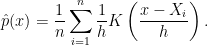
Let’s start with getting a confidence interval at a single point 
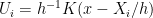
Let 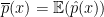


Now,

where 
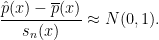
This suggests the confidence interval, 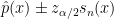
The problem is the second term 


We could in principle solve this problem by undersmoothing. If we choose a bandwidth smaller than the optimal bandwidth, then 
Of course, all of these problems are only worse when we consider simultaneous confidence band for the whole function.
The same problem arises if we use Bayesian inference. In short, the 95 percent Bayesian interval will not have 95 percent frequentist coverage. The reasons are the same as for the frequentist interval. (One can of course “declare” that coverage is not important and then there is no problem. But I am assuming that we do want correct frequentist coverage.)
The only good solution I know is to simply admit that we can’t create a confidence interval for 

where 
Once we take this point of view, we can easily get a confidence band using the bootstrap. We draw 


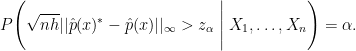
The confidence band is then 

We then have that

as 
Summary: There really is no good, practical method for getting true confidence bands in nonparametric function estimation. The reason is that the bias does not disappear fast enough as the sample size increases. The solution, I believe, is to just acknowledge that the confidence bands have a slight bias. Then we can use the bootstrap (or other methods) to compute the band. Like Dr. Strangelove, we just learn to stop worrying and love the bias.

16 Comments
Neat, Cochran noted the same problem with confidence intervals from non-randomised studies.
Unless you can bring in background/external information about the bias – your stuck with unquantified uncertainty.
hi keith, could you provide the cochran reference? much thanks!
This looks like it http://www.amazon.com/Planning-Analysis-Observational-Probability-Statistics/dp/0471887196
Though a more direct connection would be Peirce’s theory of realism where as you can’t ever get at what’s “real” or know it you can instead define what an ongoing community of (infinite) investigators would eventually settle on as being what to take as the truth.
One could wonder whether the smoothed density is a better target for inference than the true density with all kinds of potential irregularities anyway. A huge problem with densities is their striking non-robustness – in any reasonable neighbourhood of a distribution with a certain density there are distributions without density at all, or with locally arbitrarily different densities. Does anybody know whether smoothed densities (based on non-vanishing h, if necessary) are more robust in this respect?
You’re right. The mapping from a distribution to its desity is
highly discontinuous but the map to the smooth density is
continuous in the L_infinity norm.
Some actually insist on this (the mapping from the distribution to the density being continuous) to ensure that it approximates finite objects given that in statistical applications all object are finite.
I guess the core issue is that the space of densities is just too large. I don’t know much about confidence bands for densities, but for nonparametric regression if one assumes that the regression function belongs to a known smoothness class and the noise has sub-Gaussian tails with a known “sub-Gaussianity” constant, there seems to be no problem with coming up with confidence bands. An example of how this can be done is to assume that the regression function belongs to a known RKHS space. Then one may consider the ridge regression estimator that uses the squared RKHS norm. With appropriate tuning of the regularizer, this estimator will achieve the optimal rate for this given class of regression problems. Then, with some work, one can show that a confidence ellipsoid that generalizes of what would work in the finite dimensional case will still be valid and then with some algebra one can also get simultaneous confidence bands for the unknown regression function. Details of how this can be done can be found in the PhD Thesis of my former student, Yasin Abbasi-Yadkori (the thesis can be downloaded from here: https://era.library.ualberta.ca/public/datastream/get/uuid:c21661ea-0ecc-4ea8-9a9d-2b1b312a36e1/DS3, the thesis is an extension of our previous NIPS paper where we considered linear bandit problems and for these we needed the confidence bands). Although these are “honest” confidence bands, it should not be hard to “soften” these up to get confidence bands with “asymptotically correct” coverage.
Exactly the same problem happens in nonpar regression. It’s the same analysis.
You can’t get correct bands in a sobolev space without undersmoothing.
Furthermore, you can’t even adapt to the size of the Sobolev ball using the data.
See:
Mark Low (1997) Annals of Statistics, p 2547
From a quick look, it appears to me that your student constructed a confidence ball.
This does not give a band.
Theorem 3.11 in his thesis gives simultaneous confidence bands (based on the ball/ellipsoid in the RKHS). I will check out the paper, thanks for the reference.
I could be mistaken but I thought Kendall, in volume I of his series, developed a standard deviation for the median.
yes it is easy to get an exact confidence interval for the median.
But this is unrelated to function estimation.
The bootstrap examples again started with resampling from the empirical distribution of the “micro data”.
But if one is interested in a property of the density (e.g. excess mass at/around a prescpecified point) is it wrong to calculate frequencies by bins, fit some flexible parametric form, and bootstrap with resampling the error, where the error is the discrepancy between the frequency in the bin vs the predicted density? This seems to be what Chetty et al. describe on page 23 (p. 25 of the PDF) of an influential paper [1] with their posted code [2] used in other papers since.
Does this “macro level”, aggregate (block?) bootstrap do something different from resampling the empirical CDF? In any case, is the error in the parametric fit of the density the only noise we care about in the problem if we think that individual values (not frequencies) themselves have noise in them?
I also forked this comment into a question on Cross Validate [3]. Also note the related question [4] about whether the estimand is regular enough to bootstrap or subsample in the first place, and with what rate of convergence (motivated by the Normal Deviate posts from January).
[1]: http://obs.rc.fas.harvard.edu/chetty/denmark_adjcost_nber.pdf
[2]: http://obs.rc.fas.harvard.edu/chetty/bunch_count.zip
[3]: http://stats.stackexchange.com/q/69307/6534
[4]: http://stats.stackexchange.com/questions/67613/is-excess-mass-estimation-smooth-enough-to-bootstrap-at-what-rate-might-a-bunch
That seems unnecessary and kind of complicated.
And it would add additional bias.
The regular bootstrap as I described should
work fine.
Thanks! Any hints or thoughts on the source or the magnitude of the bias?
On the complication: I think the procedure was partly motivated by the preference to work on collapsed/aggregate data (much, much faster), namely frequencies by bins. You would say those are not sufficient statistics of the density, or at least the bootstrap procedure wrongly introduces within-bin correlation? (Though if all the matters is the frequency in the bin, how bad is that?)
Larry – I haven’t yet read this recent paper but it seems relevant to this discussion “A simple bootstrap method for constructing nonparametric confidence bands for functions” by Peter Hall and Joel Horowitz (http://projecteuclid.org/DPubS?service=UI&version=1.0&verb=Display&handle=euclid.aos/1378386242). I’d be interested to hear your thoughts on it if you have read it.
Thanks for the pointer
I’ll check it out
One Trackback
[…] Statistics and Dr. Strangelove (normaldeviate.wordpress.com) […]